Download
1 / 31
360 likes | 645 Views
5.3 Consumer Surplus. Difference between maximum amount a consumer is willing to pay for a good (reservation price) and the amount he must actually pay to purchase the good in the market place. 10.2 The Invisible Hand. Will always guide the supply and demand curve back to equilibrium.

E N D
5.3 Consumer Surplus Difference between maximum amount a consumer is willing to pay for a good (reservation price) and the amount he must actually pay to purchase the good in the market place.
10.2 The Invisible Hand Will always guide the supply and demand curve back to equilibrium
10.9 Import Quotas and Tariffs Pg 390 Impact of quotas and tariffs
Chapter 6 Inputs and Production Functions
Intro to Inputs and Production Functions • Inputs – Resources such as labor, capital equipment, and raw materials that are combined to produce finished goods • Factors of Production – resources that are used to produce a good • Output – The amount of a good or service produced by a firm • Production function – A mathematical representation that shows the maximum quantity of output a firm can produce given the quantities of inputs that it might employ • Q is the quantity of output Q= f(L,K) • L is the quantity of labor used • K is the quantity of capital employed • Production set – The set of technically feasible combinations of inputs and outputs
Technically Inefficient – The set of points in the productions set at which the firm is getting less output from its labor than it could • Technically Efficient – The set of points in the production set at which the firm is producing as much output as it possibly can given the amount of labor it employs • Labor requirements functions – A function that indicates the minimum amount of labor required to product a given amount of output • L=g(Q) the minimum amount of labor L required to produce a given amount of output Q
Total Product Functions • A total product function with a single input shows how total output depends on the level of the input • Increasingly marginal returns to labor – the region along the total product function where output rises with additional labor at an increasing rate (sometimes not always = to slope) • Diminishing marginal returns to labor – the region along the total product function in which output rises with additional labor but at a decreasing rate • Diminishing total returns to labor – the region along the total product function where output decreases with additional labor • Stages • 1 Increasing Marginal Returns • 2 Diminishing Marginal Returns • 3 Diminishing Total Returns
Marginal and Average Product of Labor • Average product of labor is the average output per unit of labor • APL= total product/quantity of labor = Q/L • Marginal product of labor is the rate at which total output changes as the quantity of labor the firm uses is changed. • MPL = Δ in total product/ Δ in total quantity of labor = ΔQ/ΔL
Law of diminishing marginal returns- principle The principle that as the usage of one input increases, the quantities of other inputs being held fixed, a point will be reached beyond which the marginal product of the variable input will decrease
Relationship between Marginal and Average Product • When average product is increasing in labor, marginal product is greater than average product. That is if APL increases in L, then MPL > APL • When average product is decreasing in labor, the marginal product is less than average product. That is, if APL is at maximum, then marginal product is equal to average product.
Total Product Hill A three-dimensional graph of production function
Isoquants • “Means same quantity”: any combination of labor and capital among a given isoquant allows the firm to produce the same quantity of output • Isoquant is a curve that shows all of the combinations of labor and capital that can produce given levels of output.
Economic and Uneconomic Regions of Production • Uneconomic region of production - the region of upward-sloping or backward-bending isoquants. In the uneconomic region, at least one input has a negative marginal product • Economic region of production – The region where the isoquants are downward sloping
Marginal Rate of Technical Substitution • MRTSL,K-The rate at which the quantity of capital can be reduced for every one unit increase in the quantity of labor, holding the quantity output constant. • MRTSL,K tells us: • The rate at which the quantity of capital can be decreased for every one unit increase in the quantity of labor, holding the quantity of the output constant • The rate at which the quantity of capital must be increased for every one unit decrease in the quantity of labor, holding the quantity of output constant
Diminishing Marginal Rate of Substitution A feature of a production function in which the marginal rate of technical substitution of labor for capital diminishes as the quantity of labor increases along an isoquant
Elasticity of Substitution • A measure of how easy it is for a firm to substitute labor for capital. It is equal to the percentage change in the capital-labor ratio for every one percent change in the marginal rate of technical substitution of capital for labor as we move along the isoquant • Capital-labor ratio – The ratio of the quantity of capital to the quantity of labor (used as labor is substituted by capital)
Linear Production Function • Perfect Substitutes – (in production) Inputs in a production function with a constant marginal rate of technical substitution • A production function of the form Q=aL+bK, where a and b are positive constants
The Fixed-Proportions Production Function • Fixed-proportions production function – a production function where the inputs must be combined in a constant ration to one another • Perfect complements – (in production) Inputs in a fixed-proportions production function.
The Cobb-Douglas Production Function • A production function of the form Q ALαKβ, where Q is the quantity of output from L units of labor and Kunits of capital and where A, α, and β are positive constants. • The elasticity of substitution for a Cobb–Douglas production function falls somewhere between 0 and ∞. In fact, it turns out that the elasticity of substitution along a Cobb–Douglas production function is always equal to 1. • Capital and Labor can be substituted for each other
The Constant Elasticity of Substitution Production Function A type of production function that includes linear production functions, fixed-proportions production functions, and Cobb-Douglas production functions as special cases.
Returns to Scale The concept that tells us the percentage by which output will increase when all inputs are increased by a given percentage
Let φ represent the resulting proportionate increase in the quantity of output Q (i.e., the quantity of output increases from Q to φQ). • increasing returns to scale - A proportionate increase in all input quantities resulting in a greater than proportionate increase in output. • If φ > λ • constant returns to scale - A proportionate increase in all input quantities simultaneously that results in the same percentage increase in output. • If φ = λ • decreasing returns to scale - A proportionate increase in all input quantities resulting in a less than proportionate increase in output. • φ < λ
Returns to Scale vs Diminishing Marginal Returns Returns to scale pertains to the impact of an increase in all input quantities simultaneously, while marginal returns (i.e., marginal product) pertains to the impact of an increase in the quantity of a single input, such as labor, holding the quantities of all other inputs fixed.
Technological Progress Technological Progress – a change in production process that enables a firm to achieve more output from a given combination of inputs or, equivalently, the same amount of output from less inputs
Neutral Technological Progress • progress that decreases the amounts of labor and capital needed to produce a given output, without affecting the marginal rate of technical substitution of labor for capital • or… Isoquant shifts inward indicating that lesser amounts of labor and capital are needed to produce a given output, but the shift leaves MRTSL,K, the marginal rate of technical substitution of labor or capital, unchanged along any ray (e.g., 0A) from the origin.
Labor-saving Technical Progress • progress that causes the marginal product of capital to increase relative to the marginal product of labor • Isoquant shifts inward, but the isoquant becomes flatter
Capital-Savings Technological Progress Progress that causes the marginal product of labor to increase relative to the marginal product of capital
The production function tells us the maximum quantity of output a firm can get as a function of the quantities of various inputs that it might employ. Single-input production functions are total product functions. A total product function typically has three regions: a region of increasing marginal returns, a region of diminishing marginal returns, and a region of diminishing total returns. The average product of labor is the average amount of output per unit of labor. The marginal product of labor is the rate at which total output changes as the quantity of labor a firm uses changes. The law of diminishing marginal returns says that as the usage of one input (e.g., labor) increases—the quantities of other inputs, such as capital or land, being held fixed—then at some point the marginal product of that input will decrease. Isoquants depict multiple-input production function in a two-dimensional graph. An isoquant shows all combinations of labor and capital that produce the same quantity of output. For some production functions, the isoquants have an upward-sloping and backward-bending region. This region is called the uneconomic region of production. Here, one of the inputs has a negative marginal product. The economic region of production is the region of downward-sloping isoquants. The marginal rate of technical substitution of labor for capital tells us the rate at which the quantity of capital can be reduced for every one unit increase in the quantity of labor, holding the quantity of output constant. Mathematically, the marginal rate of technical substitution of labor for capital is equal to the ratio of the marginal product of labor to the marginal product of capital. Isoquants that are bowed in toward the origin exhibit diminishing marginal rate of technical substitution. When the marginal rate of technical substitution of labor for capital diminishes, fewer and fewer units of capital can be sacrificed as each additional unit of labor is added along an isoquant. The elasticity of substitution measures the percentage rate of change of K/L for each 1 percent change in MRTSL,K. Three important special production functions are the linear production function (perfect substitutes), the fixed-proportions production function (perfect complements), and the Cobb–Douglas production function. Each of these is a member of a class of production functions known as constant elasticity of substitution production functions. Chapter Summary