Download
1 / 29
300 likes | 447 Views
Dispersion relation of the linearised shallow water equations on flat triangle/hexagon grids PDE's on the sphere 24.-27.08.2010, Potsdam Michael Baldauf , Deutscher Wetterdienst, Offenbach Almut Gassmann , Max-Planck-Institut, Hamburg Sebastian Reich , Universität Potsdam. Motivation:

E N D
Dispersion relation of the linearised shallow water equations on flat triangle/hexagon grids PDE's on the sphere 24.-27.08.2010, Potsdam Michael Baldauf, Deutscher Wetterdienst, Offenbach Almut Gassmann, Max-Planck-Institut, Hamburg Sebastian Reich, Universität Potsdam • Motivation: • Direct comparison between triangle / hexagon grids • Dispersion relation on non-equilateral grids? Correct geostrophic mode? Klemp (2009) lecture at 'PDE's on the sphere', Santa Fe Bonaventura, Klemp, Ringler (unpubl. ?)
Linearised shallow water equations analytic dispersion relation ( ): Rossby-deformation radius: LR= c / f inertial-gravity wave (Poincaré wave) geostrophic mode • 'Standard' C-grid spatial discretisation: • divergence: sum of fluxes over the edges (Gauss theorem) • gradient: centered differences ( -> 2nd order ) • Coriolis term: Reconstruction of v by next 4 neighbours with RBF-vector reconstruction (with an 'idealised' RBF-fct. =1) • temporal discretisation: assumed exact
wave analysis (x,y,t) = (kx, ky,) exp( i ( kx x + ky y - t) ) Consider arbitrary non-equilateral, however translation invariant grids consider appropriate dual hexagon grid (Voronoi tesselation) per elementary cell: 2 triangles: 3 v-components, 2 h-components 5 equations 1hexagon: 3 v-components, 1 h-component 4 equations resolution is approximately comparable translation invariance against integer linear combinations of grid vectors sufficient to plot dispersion relation in the 1st Brillouin zone
Hexagon grid analytic solution inertial- gravity wave f geostrophic mode ka 4 branches: 1,2 = ..., inertial-gravity-waves 3,4 0 false geostrophic mode with 4-point reconstruction (Nickovic et al., 2002) Thuburn (2008), Thuburn, Ringler, Skamarock, Klemp (2009): 8-point reconstruction of Coriolis term correct geostrophic mode 3,4 =0
Triangle grid main motivation: ICON-project uses local grid refinement 5 branches: 1,2 = fI-G(k), 3,4 = fHF(k), 5=0 (exact in equilat. grid!) ‚high-frequent mode‘ interpretation 1: internal excitation of an elementary cell interpretation 2: (poor) resolution of shorter waves (until 'x') ( not artificial) consequences in practice: reduction of time step 1st Brillouin-zone
Checkerboard pattern observed in triangle hydrostatic ICON … Linear shallow water test case from Gassmann (subm. to JCP) div v dim.less deformation radius: LR / a ~ 0.3 LR := (g h0)1/2 / f a : length of triangle edge time step: t ~0.1 / f 'observation': large scale checkerboard pattern in the divergence field with a oscillation frequency ~ 2 f
triangle grid: 'standard' divergence operator 1st order Eigenvalues and Eigenvectors for equilateral grid and for k=0: geostrophic mode inertial-gravity 'high-frequency' dimensionless Rossby-deformation-radius: lR= LR / a • Checkerboard oscillation in the 'high frequency' mode • in hydrostatic models for the atmosphere and in ocean models: lR << 1 can occur
Equilateral triangle and hexagon grids LR/a = 10 for different LR/a Rossby-Deform.radius LR = (g h0)1/2 / f LR/a = 0.3 a = length of triangle edge LR/a = 1 • 'high-frequency mode' • becomes 'low frequency' for badly resolved LR • group velocity = 0 for k=0 ! LR/a = 1/24 ~ 0.2 LR/a = 0.1 red: triangle grid LR/a = 1/8 ~ 0.35 blue: hexagon grid
triangle grid, equilateral a=20 km, =60°, =60°, Re() Re analytic solution (boundaries are drawn only for better comparison with grid results) inertial-gravity mode 'high-frequency mode' geostrophic mode: =0 (exact)
triangle grid, non-equilateral a=20 km, =43°, =76°, inertial-gravity mode Re analytic solution (boundaries are drawn only for better comparison with grid results) inertial-gravity mode 'high-frequency mode' geostrophic mode: =0 (numerically < 10-14 f) !
Divergence-operator 2nd order Use the nearest 9 v-positions: For equilateral triangles: g1=g2=g3=-1/3, g4=...=g9=1/6 this is identical to a weighted averaging of the divergence For an isosceles triangle grid, i.e. for = lengths l1=l5=l6=a, all other li=b and with the weights:
Divergence-operator 2nd order a=20 km, =75°, =75°, direction k=10° no 'high-frequency' mode in triangle grid! but ... apparently additional „gravity wave mode, without influence of Coriolis force“
Triangle grid: divergence operator 2nd order Eigenvector structure for equilateral grid and k=0 geostrophic mode inertial-gravity 'high-frequency' no checkerboard in height field, BUT: unphysical checkerboard in divergence !! reason: divergence-operator is 'blind' against checkerboard in velocity field otherwise: high group velocity also for k=0 unphysical disturbances travel away
Mixing: Div. 1st order (10%) + Div. 2nd order (90%) LR/a = 10 LR/a = 0.5 LR/a = 1 LR/a = 0.1
triangle grid: 3rd order divergence operator 3rd order weightings for equilateral grid: c1 = -13 / 24 - 15 c4 c2 = 29 / 144 - 5 c4 c3 = 5 / 144 eigenvector structure for k=0: geostrophic mode inertial-gravity 'high-frequency' 'non-blind' against checkerboard in divergence, if c4 > 0.
triangle grid: 3rd order divergence operator LR/a = 10 LR/a = 0.5 LR/a = 1 LR/a = 0.1
Summary • 'standard' C-griddiscretization in thetrianglegrid • produces 'high-frequent' mode • forsmall LR (ocean, hydrostaticmodels): slowlyvaryingcheckerboard in heightfield/ divergencepossible • 2nd order divergenceoperator:checkerboard in height-fieldvanishes, but unphysicalcheckerboard in v (ordiv v) due toblindnessofthediv.operator • mixingof 1st & 2nd order divergenceseemstobe a goodcompromise(seeresults in talk by Günther Zängl, Pilar Rípodas, …) • 3rd order divergenceoperator: • betterinertial-gravitywaveproperties • Non-blind against a checkerboard in v • but isitreally an alternative?
Influence of vector reconstruction up to now very broad RBF-functions were used for vector reconstruction. Now use Gauss-fct. (r)=e-r with =1/a. a=20 km, =75°, =75°, direction k=10° both triangle and hexagon don't deliver f0 at k=0
Imaginary parts of serves as a consistency check ( bug fix of vector reconstruction) a=20 km, =43°, =76°, direction k=10° Eigenvalue-solver (Lapack-routine) produces spurious imaginary parts for ~O(10-10 1/s). Are they small enough to confirm that Im =0?
a=20 km, =43°, =76°, geostrophic mode even for non-equilateral triangles, the geostrophic mode is exactly reproduced Re
Summary • triangle grid with 1st order divergence operator • [+] Inertial-gravity wave (short waves): better represented than in hexagon grid • Inertial-gravity wave (long waves): good represented (influence of vector reconstruction!) • [--] 2 artificial high frequent modes induce strong checkerboard oscillation (also reduce time step) • [++] correct geostrophic mode (=0) even for non-equilateral grids
triangle grid with 2nd order divergence operator • Günther's bilinear averaging delivers 2nd order (at least for isosceles triangles) • Inertial-gravity wave (short waves): almost identical to hexagon grid • [+] Inertial-gravity wave (long waves): good represented (influence of vector reconstruction!) • [-] no artificial high frequent modes, instead: 2 additional 'inertial-gravity-modes' without Coriolis influence (moderate checkerboard oscillation) • [++] correct geostrophic mode (=0) even for non-equilateral grids
hexagon grid • [-] Inertial-gravity wave (short waves): worse represented than in triangle grid • [+] Inertial-gravity wave (long waves): good represented (influence of vector reconstruction!) • [+] no high frequent artificial modes • false geostrophic mode (and 2 modes instead of 1) but now there exist a solution! (Thuburn; Skamarock, Klemp, Ringler)
general remarks: • (k=0) = f0 only for 'ideal' vector reconstruction;sharper RBF-functions reduce fidelity to analytic solution • for 'ideal' vector reconstruction: Im =0. • but for real vector reconstruction: Im 0 (both triangle, hexagon)
To do Divergence averaging destroys (local) conservation find 2nd order vector reconstruction method for normal fluxes (v or v) example: equilateral triangle grid: use weights: w1=2/3 w2=...=w5=1/6 • 'brute force' solution of LES possible? • Recover reconstruction method by Th. Heintze (Simpson rule) ? • Work of Jürgen Steppeler • Almuts proposal