Download
1 / 12
120 likes | 123 Views
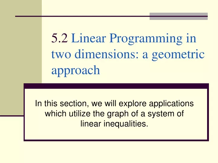
5.2 Linear Programming in two dimensions: a geometric approach. In this section, we will explore applications which utilize the graph of a system of linear inequalities. A familiar example.

E N D
5.2 Linear Programming in two dimensions: a geometric approach In this section, we will explore applications which utilize the graph of a system of linear inequalities.
A familiar example • We have seen this problem before. An extra condition will be added to make the example more interesting. Suppose a manufacturer makes two types of skis: a trick ski and a slalom ski. Suppose each trick ski requires 8 hours of design work and 4 hours of finishing. Each slalom ski 8 hours of design and 12 hours of finishing. Furthermore, the total number of hours allocated for design work is 160 and the total available hours for finishing work is 180 hours. Finally, the number of trick skis produced must be less than or equal to 15. How many trick skis and how many slalom skis can be made under these conditions? Now, here is the twist: Suppose the profit on each trick ski is $5 and the profit for each slalom ski is $10. How many each of each type of ski should the manufacturer produce to earn the greatest profit?
Linear Programming problem • This is an example of a linear programming problem. Every linear programming problem has two components: • 1. A linear objective function is to be maximized or minimized. In our case the objective function is Profit = 5x + 10y (5 dollars profit for each trick ski manufactured and $10 for every slalom ski produced). • 2. A collection of linear inequalities that must be satisfied simultaneously. These are called the constraintsof the problem because these inequalities give limitations on the values of x and y. In our case, the linear inequalities • are the constraints. x and y have to be positive The number of trick skis must be less than or equal to 15 Profit = 5x + 10y Design constraint: 8 hours to design each trick ski and 8 hours to design each slalom ski. Total design hours must be less than or equal to 160 Finishing constraint: Four hours for each trick ski and 12 hours for each slalom ski.
Linear programming • 3. Thefeasible setis the set of all points that are possible for the solution. In this case, we want to determine the value(s) of x, the number of trick skis and y, the number of slalom skis that will yield the maximum profit. Only certain points are eligible. Those are the points within the common region of intersection of the graphs of the constraining inequalities. Let’s return to the graph of the system of linear inequalities. Notice that the feasible set is the yellow shaded region. • Our task is to maximize the profit function • P = 5x + 10y by producing x trick skis and y slalom skis, but use only values of x and y that are within the yellow region graphed in the next slide.
Maximizing the profit • Profit = 5x + 10y Suppose profit equals a constant value, say k . Then the equation • k = 5x + 10y represents a family of parallel lines each with slope of one-half. For each value of k (a given profit) , there is a unique line. What we are attempting to do is to find the largest value of k possible. The graph on the next slide shows a few iso-profit lines. Every point on this profit line represents a production schedule of x and y that gives a constant profit of k dollars. As the profit k increases, the line shifts upward by the amount of increase while remaining parallel. The maximum value of profit occurs at what is called a corner point- a point of intersection of two lines. The exact point of intersection of the two lines is (7.5,12.5). Since x and y must be whole numbers, we round the answer down to (7,12). See the graph in the next slide.
Maximizing the Profit • Thus, the manufacturer should produce 7 trick skis and 12 slalom skis to achieve maximum profit. What is the maximum profit? • P = 5x + 10y P=5(7)+10(12)=35 + 120 = 155
General Result • If a linear programming problem has a solution, it is located at a vertex of the set of feasible solutions. If a linear programming problem has more than one solution, at least one of them is located at a vertex of the set of feasible solutions. • If the set of feasible solutions is bounded, as in our example, then it can be enclosed within a circle of a given radius. In these cases, the solutions of the linear programming problems will be unique. • If the set of feasible solutions is not bounded, then the solution may or may not exist. Use the graph to determine whether a solution exists or not.
General Procedure for Solving Linear Programming Problems • 1. Write an expression for the quantity that is to be maximized or minimized. This quantity is called the objective functionand will be of the form z = Ax + By. In our case z = 5x + 10y. • 2. Determine all the constraints and graph them • 3. Determine the feasible set of solutions- the set of points which satisfy all the constraints simultaneously. • 4. Determine the vertices of the feasible set. Each vertex will correspond to the point of intersection of two linear equations. So, to determine all the vertices, find these points of intersection. • 5. Determine the value of the objective function at each vertex.
Linear programming problem with no solution • Maximize the quantity z =x +2y subject to the constraints • x + y 1 , x 0 , y 0 • 1. The objective function is z = x + 2yis to be maximized. • 2. Graph the constraints: (see next slide) • 3. Determine the feasible set (see next slide) • 4. Determine the vertices of the feasible set. There are two vertices from our graph. (1,0) and (0,1) • 5. Determine the value of the objective function at each vertex. • 6. at (1,0):z = (1) + 2(0) = 1 • at (0, 1) : z = 0 + 2(1) = 2 . • We can see from the graph there is no feasible point that makes z largest. We conclude that the linear programming problem has no solution.