Download
1 / 31
430 likes | 701 Views
Introduction to EXAFS I. Scott Medling Michael Kozina Brad Car Carley Corrado Jin Zhang Yu (Justin) Jiang Lisa Downward John J. Neumeier T. Tyson Collin Broholm Satoru Nakatsuji. Outline Brief history Why EXAFS? Some general differences between local and average structure

E N D
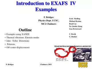
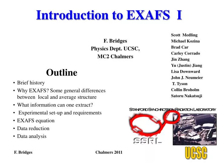
Introduction to EXAFS I Scott Medling Michael Kozina Brad Car Carley Corrado Jin Zhang Yu (Justin) Jiang Lisa Downward John J. Neumeier T. Tyson Collin Broholm Satoru Nakatsuji Outline • Brief history • Why EXAFS? Some general differences between local and average structure • What information can one extract? • Experimental set-up and requirements • EXAFS equation • Data reduction • Data analysis F. Bridges Physics Dept. UCSC, MC2 Chalmers Chalmers 2011
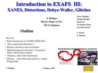
Brief History of EXAFS(Extended X-ray Absorption Fine Structure) • Every atom has well defined absorption steps. • For a solid, above each step there is structure in the absorption as a function of energy; known since ~ early ’20s-’30s Kossel , Kronig. • Many explanations proposed – some were multi-electron one was single electron (Kronig). • Stern and Sayers (Stern’s student) developed a useful model to use the oscillations to understand structure ~ 1970-71 – used Lytle’s data. • Argument as to who first suggested using Fourier Transforms will never be resolved. Chalmers 2011
What information does EXAFS provide? • Local structure about a selected atom type; determinedbyX-ray energy used. (Moseley’s Law for fluorescence) • E.g. for Cu use X-ray energies near 9000 eV; Rb, 15,200 eV; Ag, 25,500eV • Can measure bond lengths and further pair distances. Usually for bond lengths, absolute distances to 0.01Å; relative change even smaller. • Types of neighbors – but need change in Z (4 or more) • Coordination numbers – generally better than 20%; sometimes to 10%. Limited by correlations between parameters. • Disorder/Distortions – static, thermal phonons, lattice distortions (Jahn-Teller), polarons etc Bunker Chalmers 2011
Types of materials/Samples • Solids – usually complex; often distorted • Nanoparticles; small – and doped • Thin films (nano-sized grains) • Amorphous materials • Liquids (and gases); solutions • Need samples to be homogeneous and uniform in thickness. Uniform thickness – no pinholes, tapers etc., no concentration gradients. (Address in later lecture) Choose appropriate thickness for edge energy. Step height <1. Chalmers 2011
Experimental set-up for X-ray spectroscopy (solids) Side View Typical set-up for transmission µt = ln Io/I1 µReft = ln I1/I2 Source Top View Set-up for fluorescence detection. For low concentrations µ ~ If/Io Source Need very linear detectors and amps. Because use ratios, gains not important, but need dynamic range. Chalmers 2011
Typical set-up (CH Booth) double-crystal monochromator ionization detectors Leave gap between Io and sample – and I1 and sample. Keep reference sample away from I1 Reduce higher harmonics (2dsinθ = nλ) beam-stop I2 I1 I0 “white” x-rays from synchrotron LHe cryostat reference sample sample collimating slits • Windows in detectors – thin Kapton – often aluminized; 50 –75 µm . • Choose gas in detectors for energy range (He, N2, Ar, Kr, etc.) Can use mixtures to optimize. Not too much absorption in ionization detectors. • Choose edge/energy; check no other edges overlap • Prepare uniform sample Chalmers 2011
X-ray Absorption SpectroscopyExtended X-ray Absorption Fine structure (EXAFS) continuum unoccupied states EF filled 3d 1s core hole • Main features are single-electron excitations. • Away from edges, energy dependence fits a power law: AE-3+BE-4 (Victoreen). • Threshold energies E0~Z2, absorption coefficient ~Z4. • Core-hole lifetime ~ 10-15 sec sets response time – a very fast probe – but data collection slow. K-edge From G. Bunker From McMaster Tables
EXAFS /XANES overview µt = ln Io/I1 XANES Dotted background constrained by Victoreen Equ. and the step height. FT 4K Chalmers 2011
Raw absorption data, pre-edge fit • Pre-edge region –absorption from all other material in beam; includes other atom in sample. • Varies as AE-3+BE-4(Victoreen) -- tabulated in McMaster tables. • Using measured step height and Victoreen equation below edge and well above edge, can extract background above edge. • Keep step height below 1 (between 0.3 and 0.7) • Need to also know absorption from rest of sample!! Co K-edge Chalmers 2011
Pre-edge subtracted data (Co K-edge LaCoO3) • Eo – we define as the half step energy. • Slope at high energy agrees with Victoreen formula. • Errors in slope add (or subtract) to σ2. • If slope varies from trace to trace (e.g. in a temperature dependant study) get fluctuations in σ2. • EXAFS function χ(E) – the oscillations on top of a background function µo – red line. E-Eo =ħ2k2/2m Chalmers 2011
Co k-space data • Usually plot as knχ(k); here kχ(k). • Would like kmax as high as possible – but limited by noise and time to collect data. • Sum of sine waves of form • sin(2kr + Φ(k)) • Take Fourier Transform to get an r-space plot. Chalmers 2011
r-space (Co) Peaks in r-space correspond to different shells of neighbors Usually can fit out to 4-6 Å depending on the structure. EXAFS peaks shifted from real distances. Co-La Co-O Co-Co Chalmers 2011
More r-space (FT Spectra)Example: cubic ZnS:Cu,Mn • Fast oscillation – real part , R, of transform • Imaginary part , I, not shown. • Envelope function ±√(R2+ I2) • Fit to R and I • Peaks in EXAFS shifted in position by well known amount - Δr (from phase shifts δc and δb in term • sin[2kr + 2δc(k) + δb(k)] • 2δc(k) + δb(k) ≈ -2kΔr + f(k) R R Zn-Zn,; Mn-Zn Bunker Zn-S; Mn-S Chalmers 2011
continuum EF filled 3d 1s core hole X-ray Absorption Spectroscopy Time scale – 10-15 sec. “I was brought up to look at the atom as a nice hard fellow, red or grey in colour according to taste.” - Lord Rutherford Chalmers 2011
Simple model for absorption • Use Fermi’s golden rule µ ~ <f |(ε·r)2|i> • Final state f is modified by backscattering + interference of outgoing and backscattered waves, i.e. f = fo+ Δf ;dipole selection rules • Can write µ = µo(1+χ); or χ = (µ-µo)/µo µ, µo, and χ are all energy dependent Chalmers 2011
How is final state wave function modulated? From CH Booth LBL • Assume photoelectron reaches the continuum within dipole approximation: Chalmers 2011
How is final state wave function modulated? • Assume photoelectron reaches the continuum within dipole approximation: Chalmers 2011
How is final state wave function modulated? • Assume photoelectron reaches the continuum within dipole approximation: central atom phase shift c(k) Chalmers 2011
How is final state wave function modulated? • Assume photoelectron reaches the continuum within dipole approximation: central atom phase shift c(k) electronic mean-free path (k) Chalmers 2011
How is final state wave function modulated? • Assume photoelectron reaches the continuum within dipole approximation: central atom phase shift c(k) electronic mean-free path (k) complex backscattering probability f(,k) Chalmers 2011
How is final state wave function modulated? • Assume photoelectron reaches the continuum within dipole approximation: central atom phase shift c(k) electronic mean-free path (k) complex backscattering probability f(,k) complex=magnitude and phase: backscattering atom phase shift b(k) Chalmers 2011
How is final state wave function modulated? • Assume photoelectron reaches the continuum within dipole approximation: central atom phase shift c(k) electronic mean-free path (k) complex backscattering probability kf(,k) complex=magnitude and phase: backscattering atom phase shift a(k) final interference modulation per point atom! Chalmers 2011
Assumes both harmonic potential AND kσ<<1: problem at high k and/or σ(good to kσof about 1) Requires curved wave scattering, has r-dependence, use full curved wave theory: FEFF Other factors • Allow for multiple atoms Ni in a shell i and a distribution function function of bondlengths within the shell g(r) where and S02 is an inelastic loss factor Chalmers 2011
Definition of σ for Gaussian PDF • Atoms A and B displaced, can be static or dynamic. • is the second moment of the pair -distribution function. • Primarily sensitive to radial displacements • Contributions to 2 • Static distortions – distribution of pair distances from strains, impurities, etc. • Thermal phonons – Einstein or Debye models. • Polarons – a distortion associated with a partially localized charge. • An (unresolved) split peak – effective is ~ r/2 where r is the peak splitting. For uncorrelated mechanisms: σ2total= σ2static + σ2thermal+ σ2polarons+ Chalmers 2011
Fitting data I • Parameters for each shell: r, σ, N • Quantities |f(π,k)|e-2r/λ(k) and phases δc, δb calculated using program FEFF (Rehr); or obtained from experimental function for that atom-pair. • Two global parameters So2andΔEorequired when using FEFF; determined for highest amplitude data, usually at low T. ΔEo is the shift between the experimentally defined edge position and edge position where k = 0 in theory. These parameters are usually negligible when using experimental functions • Many codes are available for performing these fits: • EXCURVE98 (Diamond England) • EXAFSPAK (G. George) • IFEFFIT (M. Neville) • -SIXPACK (Sam Webb) • -ATHENA (Bruce Ravel) • GNXAS (Italy) • RSXAP (Booth, Bridges) Chalmers 2011
Fitting data II • Quandary: r-space or k-space fitting • LaCoO3 example • Since FT is a linear operator, if you do fits correctly should get same answers. • Need to define both an FT range and a range in r-space e.g. 4-14Å-1 and 1.2-2.0 Å. • Straight forward in r-space for the Co-O peak. Here one fits a model to the real and imaginary parts of FT over a restricted range in r-space. • k-space?? If fit the model for the Co-O peak to the full k-space data, poor fit. • The other components (other peaks) act like noise or an oscillating background • Need to go to r-space, and then back-transform the region of interest (Co-O peak) into k-space. Chalmers 2011
4 K La/Sr 300 K O Co Example of a fit – first peak;Co-O • Fit r-range, 1.1 – 1.6 Å; k-range 3.3 – 13 Å-1. • Space group R-3c is used to calculate theoretical Co-O function using FEFF code. • From the fit, we extract the width, σ, of the PDF of the Co-O bond; σ = 0.059 Å • Its bond length (1.92 Å) agrees well with diffraction results, ~ 0.01 Å. • Below 1 Å, often poor agreement – all errors in background subtractions etc. , end up in this low r range. • Region between 1.8 and 2.2 Å, interference between 1st and 2nd neighbors Nearly cubic (trigonal), Co-O-Co 163-167° Chalmers 2011
Some caveats • Many places to develop systematic errors - pre-edge subtraction and using multiple splines to obtain µo are two main areas for such errors. Errors in pre-edge subtraction can lead to error in σ. • Using multiple splines is a type of filter. Want to extract any slow variation in background (part of µo) but don’t want to also filter out part of EXAFS. Termination of spline fit near edge is very important. A spline is a cubic polynomial fit over a restricted range. For multiple splines, match value and slope where two splines join. Chalmers 2011
Further reading • Overviews: • B. K. Teo, “EXAFS: Basic Principles and Data Analysis” (Springer, New York, 1986). • Hayes and Boyce, Solid State Physics 37, 173 (1982). • “X-Ray Absorption: Principles, Applications, Techniques of EXAFS, SEXAFS and XANES”, ed. by Koningsberger and Prins (Wiley, New York, 1988). • Historically important: • Sayers, Stern, Lytle, Phys. Rev. Lett. 71, 1204 (1971). • History: • Lytle, J. Synch. Rad. 6, 123 (1999). (http://www.exafsco.com/techpapers/index.html) • Stumm von Bordwehr, Ann. Phys. Fr. 14, 377 (1989). • Theory papers of note: • Lee, Phys. Rev. B 13, 5261 (1976). • Rehr and Albers, Rev. Mod. Phys. 72, 621 (2000). • Useful links • xafs.org (especially see Tutorials section) • http://www.i-x-s.org/ (International XAS society) • http://www.csrri.iit.edu/periodic-table.html (absorption calculator)
More caveats II • Don’t go too low in k-space in choosing the FT range. Remember k = 0.512 (E-Eo)½; so for k = 3 Å-1 , E-Eo= 34.3 3V, and for k = 2 Å-1, E-Eo= 15.3 eV. XANES structure usually extends up to 20-30 eV above edge and sometimes higher, so dangerous to go below k = 3 Å-1. If not sure, do fits for various FT ranges- parameters should not change significantly. If large change in σ, say from kmin = 2.5 and 3 Å-1 then a problem. • Strong correlations between N and σ. Don’t think of σ as a “throw-away” parameter, even when you are more interested in N and r. σ must be larger than zero-point motion value. • kn weighting; depends on backscattering atom. Usually k2 or k3 make EXAFS spectra sharper – but be careful of noise at high k. Chalmers 2011
A view of Monterey bay from above UCSC Chalmers 2011