Download
1 / 53
540 likes | 724 Views
Computer Architecture Lec 3 – Performance + Pipeline Review. Review from last lecture. Tracking and extrapolating technology part of architect’s responsibility Expect Bandwidth in disks, DRAM, network, and processors to improve by at least as much as the square of the improvement in Latency

E N D
Lec 02-intro Review from last lecture • Tracking and extrapolating technology part of architect’s responsibility • Expect Bandwidth in disks, DRAM, network, and processors to improve by at least as much as the square of the improvement in Latency • Quantify Cost (vs. Price) • IC f(Area2) + Learning curve, volume, commodity, margins • Quantify dynamic and static power • Capacitance x Voltage2 x frequency, Energy vs. power • Quantify dependability • Reliability (MTTF vs. FIT), Availability (MTTF/(MTTF+MTTR)
Lec 02-intro Outline • Review • Quantify and summarize performance • Ratios, Geometric Mean, Multiplicative Standard Deviation • F&P: Benchmarks age, disks fail,1 point fail danger • 252 Administrivia • MIPS – An ISA for Pipelining • 5 stage pipelining • Structural and Data Hazards • Forwarding • Branch Schemes • Exceptions and Interrupts • Conclusion
Lec 02-intro performance(x) = 1 execution_time(x) Performance(X) Execution_time(Y) n = = Performance(Y) Execution_time(X) Definition: Performance • Performance is in units of things per sec • bigger is better • If we are primarily concerned with response time " X is n times faster than Y" means
Lec 02-intro Performance: What to measure • Usually rely on benchmarks vs. real workloads • To increase predictability, collections of benchmark applications-- benchmark suites -- are popular • SPECCPU: popular desktop benchmark suite • CPU only, split between integer and floating point programs • SPECint2000 has 12 integer, SPECfp2000 has 14 integer pgms • SPECCPU2006 to be announced Spring 2006 • SPECSFS (NFS file server) and SPECWeb (WebServer) added as server benchmarks • Transaction Processing Council measures server performance and cost-performance for databases • TPC-C Complex query for Online Transaction Processing • TPC-H models ad hoc decision support • TPC-W a transactional web benchmark • TPC-App application server and web services benchmark
Lec 02-intro How Summarize Suite Performance (1/5) • Arithmetic average of execution time of all pgms? • But they vary by 4X in speed, so some would be more important than others in arithmetic average • Could add a weights per program, but how pick weight? • Different companies want different weights for their products • SPECRatio: Normalize execution times to reference computer, yielding a ratio proportional to performance = time on reference computer time on computer being rated
How Summarize Suite Performance (2/5) • If program SPECRatio on Computer A is 1.25 times bigger than Computer B, then • Note that when comparing 2 computers as a ratio, execution times on the reference computer drop out, so choice of reference computer is irrelevant Lec 02-intro
How Summarize Suite Performance (3/5) • Since ratios, proper mean is geometric mean (SPECRatio unitless, so arithmetic mean meaningless) • 2 points make geometric mean of ratios attractive to summarize performance: • Geometric mean of the ratios is the same as the ratio of the geometric means • Ratio of geometric means = Geometric mean of performance ratios choice of reference computer is irrelevant! Lec 02-intro
How Summarize Suite Performance (4/5) • Does a single mean well summarize performance of programs in benchmark suite? • Can decide if mean a good predictor by characterizing variability of distribution using standard deviation • Like geometric mean, geometric standard deviation is multiplicative rather than arithmetic • Can simply take the logarithm of SPECRatios, compute the standard mean and standard deviation, and then take the exponent to convert back: Lec 02-intro
How Summarize Suite Performance (5/5) • Standard deviation is more informative if know distribution has a standard form • bell-shaped normal distribution, whose data are symmetric around mean • lognormal distribution, where logarithms of data--not data itself--are normally distributed (symmetric) on a logarithmic scale • For a lognormal distribution, we expect that 68% of samples fall in range 95% of samples fall in range • Note: Excel provides functions EXP(), LN(), and STDEV() that make calculating geometric mean and multiplicative standard deviation easy Lec 02-intro
log-normal distribution is a probability distribution of a random variable whose logarithm is normally distributed Lec 02-intro
Outside 1 StDev Example Standard Deviation (1/2) • GM and multiplicative StDev of SPECfp2000 for Itanium 2 Lec 02-intro
Outside 1 StDev Example Standard Deviation (2/2) • GM and multiplicative StDev of SPECfp2000 for AMD Athlon Lec 02-intro
Lec 02-intro Comments on Itanium 2 and Athlon • Standard deviation of 1.98 for Itanium 2 is much higher-- vs. 1.40--so results will differ more widely from the mean, and therefore are likely less predictable • SPECRatios falling within one standard deviation: • 10 of 14 benchmarks (71%) for Itanium 2 • 11 of 14 benchmarks (78%) for Athlon • Thus, results are quite compatible with a lognormal distribution (expect 68% for 1 StDev)
Lec 02-intro Fallacies and Pitfalls (1/2) • Fallacies - commonly held misconceptions • When discussing a fallacy, we try to give a counterexample. • Pitfalls - easily made mistakes. • Often generalizations of principles true in limited context • Show Fallacies and Pitfalls to help you avoid these errors • Fallacy: Benchmarks remain valid indefinitely • Once a benchmark becomes popular, tremendous pressure to improve performance by targeted optimizations or by aggressive interpretation of the rules for running the benchmark: “benchmarksmanship.” • 70 benchmarks from the 5 SPEC releases. 70% were dropped from the next release since no longer useful • Pitfall: A single point of failure • Rule of thumb for fault tolerant systems: make sure that every component was redundant so that no single component failure could bring down the whole system (e.g, power supply)
Lec 02-intro Fallacies and Pitfalls (2/2) • Fallacy - Rated MTTF of disks is 1,200,000 hours or 140 years, so disks practically never fail • But disk lifetime is 5 years replace a disk every 5 years; on average, 28 replacements wouldn't fail • A better unit: % that fail (1.2M MTTF = 833 FIT) • Fail over lifetime: if had 1000 disks for 5 years= 1000*(5*365*24)*833 /109 = 36,485,000 / 106 = 37 = 3.7% (37/1000) fail over 5 yr lifetime (1.2M hr MTTF) • But this is under pristine conditions • little vibration, narrow temperature range no power failures • Real world: 3% to 6% of SCSI drives fail per year • 3400 - 6800 FIT or 150,000 - 300,000 hour MTTF [Gray & van Ingen 05] • 3% to 7% of ATA drives fail per year • 3400 - 8000 FIT or 125,000 - 300,000 hour MTTF [Gray & van Ingen 05]
Lec 02-intro Outline • Review • Quantify and summarize performance • Ratios, Geometric Mean, Multiplicative Standard Deviation • F&P: Benchmarks age, disks fail,1 point fail danger • 252 Administrivia • MIPS – An ISA for Pipelining • 5 stage pipelining • Structural and Data Hazards • Forwarding • Branch Schemes • Exceptions and Interrupts • Conclusion
Lec 02-intro A "Typical" RISC ISA • 32-bit fixed format instruction (3 formats) • 32 32-bit GPR (R0 contains zero, DP take pair) • 3-address, reg-reg arithmetic instruction • Single address mode for load/store: base + displacement • no indirection • Simple branch conditions • Delayed branch see: SPARC, MIPS, HP PA-Risc, DEC Alpha, IBM PowerPC, CDC 6600, CDC 7600, Cray-1, Cray-2, Cray-3
Lec 02-intro Example: MIPS ( MIPS) Register-Register 6 5 11 10 31 26 25 21 20 16 15 0 Op Rs1 Rs2 Rd Opx Register-Immediate 31 26 25 21 20 16 15 0 immediate Op Rs1 Rd Branch 31 26 25 21 20 16 15 0 immediate Op Rs1 Rs2/Opx Jump / Call 31 26 25 0 target Op
Lec 02-intro signals Datapath vs Control Datapath Controller • Datapath: Storage, FU, interconnect sufficient to perform the desired functions • Inputs are Control Points • Outputs are signals • Controller: State machine to orchestrate operation on the data path • Based on desired function and signals Control Points
Lec 02-intro Approaching an ISA • Instruction Set Architecture • Defines set of operations, instruction format, hardware supported data types, named storage, addressing modes, sequencing • Meaning of each instruction is described by RTL on architected registers and memory • Given technology constraints assemble adequate datapath • Architected storage mapped to actual storage • Function units to do all the required operations • Possible additional storage (eg. MAR, MBR, …) • Interconnect to move information among regs and FUs • Map each instruction to sequence of RTLs • Collate sequences into symbolic controller state transition diagram (STD) • Lower symbolic STD to control points • Implement controller
Lec 02-intro Adder 4 Address Inst ALU 5 Steps of MIPS DatapathFigure A.2, Page A-8 Instruction Fetch Instr. Decode Reg. Fetch Execute Addr. Calc Memory Access Write Back Next PC MUX Next SEQ PC Zero? RS1 Reg File MUX RS2 Memory Data Memory L M D RD MUX MUX Sign Extend IR <= mem[PC]; PC <= PC + 4 Imm WB Data Reg[IRrd] <= Reg[IRrs] opIRop Reg[IRrt]
Lec 02-intro IF/ID ID/EX EX/MEM MEM/WB Adder 4 Address ALU 5 Steps of MIPS DatapathFigure A.3, Page A-9 Instruction Fetch Execute Addr. Calc Memory Access Instr. Decode Reg. Fetch Write Back Next PC MUX Next SEQ PC Next SEQ PC Zero? RS1 Reg File MUX Memory RS2 Data Memory MUX MUX IR <= mem[PC]; PC <= PC + 4 Sign Extend WB Data Imm A <= Reg[IRrs]; B <= Reg[IRrt] RD RD RD rslt <= A opIRop B WB <= rslt Reg[IRrd] <= WB
Lec 02-intro jmp br LD RI r <= A + IRim r <= A opIRop IRim if bop(A,b) PC <= PC+IRim PC <= IRjaddr WB <= r WB <= Mem[r] Reg[IRrd] <= WB Reg[IRrd] <= WB Inst. Set Processor Controller IR <= mem[PC]; PC <= PC + 4 Ifetch opFetch-DCD A <= Reg[IRrs]; B <= Reg[IRrt] JSR JR ST RR r <= A opIRop B WB <= r Reg[IRrd] <= WB
Lec 02-intro IF/ID ID/EX EX/MEM MEM/WB Adder 4 Address ALU 5 Steps of MIPS DatapathFigure A.3, Page A-9 Instruction Fetch Execute Addr. Calc Memory Access Instr. Decode Reg. Fetch Write Back Next PC MUX Next SEQ PC Next SEQ PC Zero? RS1 Reg File MUX Memory RS2 Data Memory MUX MUX Sign Extend WB Data Imm RD RD RD • Data stationary control • local decode for each instruction phase / pipeline stage
Lec 02-intro Cycle 1 Cycle 2 Cycle 3 Cycle 4 Cycle 5 Cycle 6 Cycle 7 Reg ALU Reg Ifetch DMem Reg ALU Reg Ifetch DMem Reg ALU Reg Ifetch DMem Reg ALU Reg Ifetch DMem Visualizing PipeliningFigure A.2, Page A-8 Time (clock cycles) I n s t r. O r d e r
Lec 02-intro Pipelining is not quite that easy! • Limits to pipelining: Hazards prevent next instruction from executing during its designated clock cycle • Structural hazards: HW cannot support this combination of instructions (single person to fold and put clothes away) • Data hazards: Instruction depends on result of prior instruction still in the pipeline (missing sock) • Control hazards: Caused by delay between the fetching of instructions and decisions about changes in control flow (branches and jumps).
Lec 02-intro Reg ALU Reg Ifetch Reg ALU Reg Ifetch DMem Reg ALU Reg Ifetch DMem Reg ALU Reg DMem Reg ALU Reg Ifetch DMem One Memory Port/Structural HazardsFigure A.4, Page A-14 Time (clock cycles) Cycle 1 Cycle 2 Cycle 3 Cycle 4 Cycle 5 Cycle 6 Cycle 7 I n s t r. O r d e r Load DMem Instr 1 Instr 2 Instr 3 Ifetch Instr 4
Lec 02-intro Reg ALU Reg Ifetch Reg ALU Reg Ifetch DMem Reg ALU Reg Ifetch DMem Bubble Bubble Bubble Bubble Bubble Reg ALU Reg Ifetch DMem One Memory Port/Structural Hazards(Similar to Figure A.5, Page A-15) Time (clock cycles) Cycle 1 Cycle 2 Cycle 3 Cycle 4 Cycle 5 Cycle 6 Cycle 7 I n s t r. O r d e r Load DMem Instr 1 Instr 2 Stall Instr 3 How do you “bubble” the pipe?
Lec 02-intro Speed Up Equation for Pipelining For simple RISC pipeline, CPI = 1:
Lec 02-intro Example: Dual-port vs. Single-port • Machine A: Dual ported memory (“Harvard Architecture”) • Machine B: Single ported memory, but its pipelined implementation has a 1.05 times faster clock rate • Ideal CPI = 1 for both • Loads are 40% of instructions executed SpeedUpA = Pipeline Depth/(1 + 0) x (clockunpipe/clockpipe) = Pipeline Depth SpeedUpB = Pipeline Depth/(1 + 0.4 x 1) x (clockunpipe/(clockunpipe / 1.05) = (Pipeline Depth/1.4) x 1.05 = 0.75 x Pipeline Depth SpeedUpA / SpeedUpB = Pipeline Depth/(0.75 x Pipeline Depth) = 1.33 • Machine A is 1.33 times faster
Lec 02-intro EX WB MEM IF ID/RF I n s t r. O r d e r add r1,r2,r3 Reg ALU Reg Ifetch DMem sub r4,r1,r3 Reg ALU Reg Ifetch DMem and r6,r1,r7 Reg ALU Reg Ifetch DMem or r8,r1,r9 Reg ALU Reg Ifetch DMem xor r10,r1,r11 Reg ALU Reg Ifetch DMem Data Hazard on R1Figure A.6, Page A-17 Time (clock cycles)
Lec 02-intro Three Generic Data Hazards • Read After Write (RAW)InstrJ tries to read operand before InstrI writes it • Caused by a “Dependence” (in compiler nomenclature). This hazard results from an actual need for communication. I: add r1,r2,r3 J: sub r4,r1,r3
Lec 02-intro Three Generic Data Hazards I: sub r4,r1,r3 J: add r1,r2,r3 K: mul r6,r1,r7 • Write After Read (WAR)InstrJ writes operand before InstrI reads it • Called an “anti-dependence” by compiler writers.This results from reuse of the name “r1”. • Can’t happen in MIPS 5 stage pipeline because: • All instructions take 5 stages, and • Reads are always in stage 2, and • Writes are always in stage 5
Lec 02-intro I: sub r1,r4,r3 J: add r1,r2,r3 K: mul r6,r1,r7 Three Generic Data Hazards • Write After Write (WAW)InstrJ writes operand before InstrI writes it. • Called an “output dependence” by compiler writersThis also results from the reuse of name “r1”. • Can’t happen in MIPS 5 stage pipeline because: • All instructions take 5 stages, and • Writes are always in stage 5 • Will see WAR and WAW in more complicated pipes
Lec 02-intro I n s t r. O r d e r add r1,r2,r3 Reg ALU Reg Ifetch DMem sub r4,r1,r3 Reg ALU Reg Ifetch DMem Reg ALU and r6,r1,r7 Reg Ifetch DMem Reg ALU or r8,r1,r9 Reg Ifetch DMem Reg ALU Reg Ifetch DMem xor r10,r1,r11 Forwarding to Avoid Data HazardFigure A.7, Page A-19 Time (clock cycles)
Lec 02-intro ALU HW Change for ForwardingFigure A.23, Page A-37 ID/EX EX/MEM MEM/WR NextPC mux Registers Data Memory mux mux Immediate What circuit detects and resolves this hazard?
Lec 02-intro I n s t r. O r d e r add r1,r2,r3 Reg ALU Reg Ifetch DMem lw r4, 0(r1) Reg ALU Reg Ifetch DMem Reg ALU sw r4,12(r1) Reg Ifetch DMem Reg ALU or r8,r6,r9 Reg Ifetch DMem Reg ALU Reg Ifetch DMem xor r10,r9,r11 Forwarding to Avoid LW-SW Data HazardFigure A.8, Page A-20 Time (clock cycles)
Lec 02-intro lwr1, 0(r2) I n s t r. O r d e r Reg ALU Reg Ifetch DMem sub r4,r1,r6 Reg ALU Reg Ifetch DMem ALU and r6,r1,r7 Reg Reg Ifetch DMem Reg ALU Reg or r8,r1,r9 Ifetch DMem Data Hazard Even with ForwardingFigure A.9, Page A-21 Time (clock cycles)
Lec 02-intro Reg ALU Reg Ifetch DMem Bubble Reg ALU Reg Ifetch DMem Bubble Reg Reg ALU Ifetch DMem Ifetch Reg Data Hazard Even with Forwarding(Similar to Figure A.10, Page A-21) Time (clock cycles) I n s t r. O r d e r lwr1, 0(r2) sub r4,r1,r6 and r6,r1,r7 Bubble ALU DMem or r8,r1,r9 How is this detected?
Lec 02-intro Software Scheduling to Avoid Load Hazards Fast code: LW Rb,b LW Rc,c LW Re,e ADD Ra,Rb,Rc LW Rf,f SW a,Ra SUB Rd,Re,Rf SW d,Rd Try producing fast code for a = b + c; d = e – f; assuming a, b, c, d ,e, and f in memory. Slow code: LW Rb,b LW Rc,c ADD Ra,Rb,Rc SW a,Ra LW Re,e LW Rf,f SUB Rd,Re,Rf SW d,Rd Compiler optimizes for performance. Hardware checks for safety.
Lec 02-intro Outline • Review • Quantify and summarize performance • Ratios, Geometric Mean, Multiplicative Standard Deviation • F&P: Benchmarks age, disks fail,1 point fail danger • MIPS – An ISA for Pipelining • 5 stage pipelining • Structural and Data Hazards • Forwarding • Branch Schemes • Exceptions and Interrupts • Conclusion
Lec 02-intro 10: beq r1,r3,36 Reg ALU Reg Ifetch DMem 14: and r2,r3,r5 Reg ALU Reg Ifetch DMem 18: or r6,r1,r7 Reg ALU Reg Ifetch DMem 22: add r8,r1,r9 Reg ALU Reg Ifetch DMem 36: xor r10,r1,r11 Reg ALU Reg Ifetch DMem Control Hazard on BranchesThree Stage Stall What do you do with the 3 instructions in between? How do you do it? Where is the “commit”?
Lec 02-intro Branch Stall Impact • If CPI = 1, 30% branch, Stall 3 cycles => new CPI = 1.9! • Two part solution: • Determine branch taken or not sooner, AND • Compute taken branch address earlier • MIPS branch tests if register = 0 or 0 • MIPS Solution: • Move Zero test to ID/RF stage • Adder to calculate new PC in ID/RF stage • 1 clock cycle penalty for branch versus 3
Lec 02-intro EX/MEM MEM/WB ID/EX IF/ID Adder 4 Address ALU Pipelined MIPS DatapathFigure A.24, page A-38 Instruction Fetch Execute Addr. Calc Memory Access Instr. Decode Reg. Fetch Write Back Next SEQ PC Next PC MUX Adder Zero? RS1 Reg File Memory RS2 Data Memory MUX MUX Sign Extend WB Data Imm RD RD RD • Interplay of instruction set design and cycle time.
Lec 02-intro Four Branch Hazard Alternatives #1: Stall until branch direction is clear #2: Predict Branch Not Taken • Execute successor instructions in sequence • “Squash” instructions in pipeline if branch actually taken • Advantage of late pipeline state update • 47% MIPS branches not taken on average • PC+4 already calculated, so use it to get next instruction #3: Predict Branch Taken • 53% MIPS branches taken on average • But haven’t calculated branch target address in MIPS • MIPS still incurs 1 cycle branch penalty • Other machines: branch target known before outcome
Lec 02-intro Four Branch Hazard Alternatives #4: Delayed Branch • Define branch to take place AFTER a following instruction branch instruction sequential successor1 sequential successor2 ........ sequential successorn branch target if taken • 1 slot delay allows proper decision and branch target address in 5 stage pipeline • MIPS uses this Branch delay of length n
Lec 02-intro becomes becomes becomes if $2=0 then add $1,$2,$3 if $1=0 then add $1,$2,$3 sub $4,$5,$6 add $1,$2,$3 if $1=0 then sub $4,$5,$6 Scheduling Branch Delay Slots (Fig A.14) A. From before branch B. From branch target C. From fall through add $1,$2,$3 if $1=0 then add $1,$2,$3 if $2=0 then • A is the best choice, fills delay slot & reduces instruction count (IC) • In B, the sub instruction may need to be copied, increasing IC • In B and C, must be okay to execute sub when branch fails sub $4,$5,$6 delay slot delay slot add $1,$2,$3 if $1=0 then sub $4,$5,$6 delay slot
Lec 02-intro Delayed Branch • Compiler effectiveness for single branch delay slot: • Fills about 60% of branch delay slots • About 80% of instructions executed in branch delay slots useful in computation • About 50% (60% x 80%) of slots usefully filled • Delayed Branch downside: As processor go to deeper pipelines and multiple issue, the branch delay grows and need more than one delay slot • Delayed branching has lost popularity compared to more expensive but more flexible dynamic approaches • Growth in available transistors has made dynamic approaches relatively cheaper
Lec 02-intro Evaluating Branch Alternatives Assume 4% unconditional branch, 6% conditional branch- untaken, 10% conditional branch-taken Scheduling Branch CPI speedup v. speedup v. scheme penalty unpipelined stall Stall pipeline 3 1.60 3.1 1.0 Predict taken 1 1.20 4.2 1.33 Predict not taken 1 1.14 4.4 1.40 Delayed branch 0.5 1.10 4.5 1.45