Download
1 / 42
420 likes | 699 Views
CS490 Chapter 7b, Leon-Garcia. Packet Switching Networks. 7.3 Datagrams vs. Virtual Circuits (a little more) Plus Definition of ATM 7.4 Routing in Packet Networks Distance Vector, Link State, Flooding, Deflection Routing, Source Routing 7.5 Shortest Path Algorithms Bellman Ford Algorithm

E N D
CS490Chapter 7b, Leon-Garcia Packet Switching Networks
7.3 Datagrams vs. Virtual Circuits (a little more) Plus Definition of ATM 7.4 Routing in Packet Networks Distance Vector, Link State, Flooding, Deflection Routing, Source Routing 7.5 Shortest Path Algorithms Bellman Ford Algorithm Construction of Routing Table and Updates (On the blackboard) We will not cover Dijkstra's algorithm in detail Today’s Outline
Messages Messages Segments Transport layer Transport layer Network service Network service Network layer Network layer Network layer Network layer End system b End system a Data link layer Data link layer Data link layer Data link layer Physical layer Physical layer Physical layer Physical layer Figure 7.2
3 2 2 3 2 2 2 2 2 2 2 2 1 1 2 2 2 1 1 1 1 1 1 1 2 1 1 1 1 1 3 3 4 C 3 End system b End system a 4 4 3 3 Medium B A Network 1 Physical layer entity Network layer entity Network layer entity Data link layer entity Transport layer entity 2 Figure 7.3
Actually most information on IP is in Chapter 8 on TCP/IP Here we should just know that IP is a datagram service, packets are routed independently of one another It is not connection-oriented at the network layer, but can be at the transport layer above The IP packet has a header of 20-60 bytes including source and destination addresses, CRC, and various option and control fields. Details in 8.2. The total length of a packet, including info, can be up to 65K bytes, but transit of Ethernet LANs often limits to 1500 bytes IP Internet Protocol (Network Layer)
We will skip 7.6 as far as the exam is concerned, but here is a concise definition of ATM (p 483) Connection oriented in network layer Short (48 info bytes) fixed length packets called “cells” Cells contain short (5 byte) headers that point to connections ATM uses fast hardware switches up to 10,000 ports with up to 150Mbps each ATM has some of the best features of circuit switching and packet switching. Asychronous = no master clock Asynchronous Transfer Mode Definition
Combinations of Service and Subnet Structure Type of Subnet (Network Layer)
Net = Routers (or Switches) and links Routing involves Setting up routing tables Forwarding packets Routing Algorithm tries to set up “best” routes minimize hops or minimize delay or maximize bandwidth or ... The Routing Algorithm needs global info about net 7.4 Routing in Packet Switched Networks
Rapid and Accurate Delivery of Packets Adapt to Failure of Node or Link Adapt to Change in Traffic Loads Determine Connectivity of Network Low Overhead Goals of Routing Algorithm
Static vs. Dynamic (Adaptive) Centralized vs. Distributed Decisions for each Packet vs. at Connection Time Classification of Routing Algorithms
Example of a Packet-Switched Network: Topology for Example 1 3 6 A 4 B Host 2 Switch or router 5 Figure 7.23
Virtual Circuit Packet Switching 2 7 1 8 B 1 3 3 A 1 6 5 5 4 2 4 3 5 2 C 5 6 D 2 Note: VC numbers change at each router. Route on top (thin line) changes from 1 to 2 to 7 to 8. Next slide has routing tables. Figure 7.24
Follow that circuit from A via VC Nos. 1, 2, 7,8 to B in Routers 1, 3, and 6. Node 3 Incoming Outgoing Node 6 Node 1 node VC node VC 1 2 6 7 Incoming Outgoing Incoming Outgoing 1 3 4 4 node VC node VC node VC node VC 4 2 6 1 3 7 B 8 A 1 3 2 6 7 1 2 3 1 B 5 A 5 3 3 6 1 4 2 B 5 3 1 3 2 A 1 4 4 1 3 B 8 3 7 3 3 A 5 Node 4 Incoming Outgoing node VC node VC 2 3 3 2 Node 2 Node 5 3 4 5 5 Incoming Outgoing Incoming Outgoing 3 2 2 3 node VC node VC node VC node VC 5 5 3 4 C 6 4 3 4 5 D 2 4 3 C 6 D 2 4 5 Figure 7.25
Routing Tables for a Datagram Network. Same Topology. Node 3 Destination Next node Node 6 Node 1 Destination Next node 1 1 Destination Next node 2 4 1 3 2 2 4 4 2 5 3 3 5 6 3 3 4 4 6 6 4 3 5 2 5 5 6 3 Node 4 Destination Next node 1 1 2 2 Node 2 Node 5 3 3 Destination Next node Destination Next node 5 5 1 1 1 4 6 3 3 1 2 2 4 4 3 4 5 5 4 4 6 5 6 6 Figure 7.26
Actually the book covers TCP/IP together in Chapter 8 Here (p 488) it points out that routing is simplified if hosts within a domain have the same prefix (network address). Then routers outside the domain only have to examine (and store) the prefix Thus IP addresses are always divided into a network address and a host address. (Usually there are three levels, often: network address, LAN address, host address) See Fig 7.27 Hierarchical Addresses in the Internet
0000 0001 0010 0011 0011 0110 1001 1100 0011 0101 1000 1111 0000 0111 1010 1101 0001 0100 1011 1110 0100 0101 0110 0111 1100 1101 1110 1111 1000 1001 1010 1011 R2 R2 R1 R1 Fig. 7.27 Advantage of Hierarchical Routing (a) 1 4 3 a. Hierarchical - 5 2 00 1 01 3 10 2 11 3 00 3 01 4 10 3 11 5 (b) 1 4 3 b. Non - Hier. 5 2 0001 4 0100 4 1011 4 … … 0000 1 0111 1 1010 1 … … Figure 7.27
Fig. 7.28 Sample net with costs. We will use this net for a detailed example on the blackboard 2 1 1 3 6 5 2 3 4 1 2 3 2 5 4 But, first let's finish talking about different types of routing. Figure 7.28
Results of Bellman-Ford Algorithm: Shortest path tree for this network. 2 1 1 3 6 2 4 1 2 2 5 Our bird's eye view of the net allows us to easily see that this is the lowest cost solution, but it's not so easy for the routers to do this automatically. They only have information measured by other routers to use. Figure 7.29
Distance Vector (original Internet approach, uses only one metric, often hops, uses Bellman-Ford, has count-to-infinity problem, RIP still used in internets) Link State (now most common in Internet, uses Dijkstra,can use multiple cost functions, avoids count-to-infinity) Shortest Path Routing Approaches
Flooding Deflection Routing Source Routing Other Routing Approaches
1 3 6 4 2 5 Flooding Routing Algorithm (a) Send incoming packets on all output ports, except the one it came in on. First step. Figure 7.33 - Part 1 of 3
1 3 6 4 2 5 Second Step of Flooding (b) Figure 7.33 - Part 2 of 3
1 3 6 4 2 5 Third step of Flooding. Need control to prevent saturation of network. Use "time-to-live" field (c) Figure 7.33 - Part 3 of 3
Hot Potato or Deflection Routing 0,0 0,1 0,2 0,3 1,0 1,1 1,2 1,3 2,0 2,1 2,2 2,3 3,0 3,1 3,2 3,3 Figure 7.34
Routers can do without buffers. Pure switch can be used. busy 0,0 0,1 0,2 0,3 1,0 1,1 1,2 1,3 2,0 2,1 2,2 2,3 3,0 3,1 3,2 3,3 (0,2) wants to send to (1,0), but (0,1) is busy. Deflect to right. Figure 7.35
1,3,6,B Source Routing 3,6,B 6,B 1 3 B 6 A 4 B Source host 2 Destination host 5 Figure 7.36
Congestion 3 6 1 4 8 2 7 5 Figure 7.50
Controlled Throughput Uncontrolled Offered load Figure 7.51
Peak rate Bits per second Average rate Time Figure 7.52
Water poured irregularly Leaky bucket Water drains at a constant rate Figure 7.53
Arrival of a packet at time ta X’ = X - (ta - LCT) Yes X’ < 0? No X’ = 0 Yes Nonconforming X’ > L? packet No X = X’ + I X = value of the leaky bucket counter LCT = ta X’ = auxiliary variable conforming packet LCT = last conformance time Figure 7.54
Nonconforming Packet arrival Time L+I Bucket content I Time * * * * * * * * * Figure 7.55
MBS Time T L I Figure 7.56
Leaky bucket 1 PCR and CDVT Tagged or dropped Incoming traffic Untagged traffic Leaky bucket 2 SCR and MBS Tagged or dropped Untagged traffic Figure 7.57
10 Kbps (a) 0 1 2 3 Time 50 Kbps (b) 0 1 2 3 Time 100 Kbps (c) 0 1 2 3 Time Figure 7.58
Shaped Incoming Size N traffic traffic Server Packet Figure 7.59
Tokens arrive periodically Size K Token Shaped Incoming Size N traffic traffic Server Packet Figure 7.60
b bytes instantly r bytes per second t Figure 7.61
A(t) = b+rt (a) No backlog of packets R(t) R(t) (b) b R - r Buffer occupancy @ 1 empty t bR t 0 Figure 7.62
Congestion occurs Congestion 20 avoidance 15 Congestion window Threshold 10 Slow start 5 0 Round-trip times Figure 7.63
3 2 2 3 2 2 2 2 2 2 2 2 1 1 2 2 2 1 1 1 1 1 1 1 2 1 1 1 1 1 3 3 4 C 3 End system b End system a 4 4 3 3 Medium B A Network 1 Physical layer entity Network layer entity Network layer entity Data link layer entity Transport layer entity 2 Figure 7.3