Download
1 / 37
370 likes | 504 Views
Snow and ice in polar and sub-polar seas: numerical modeling and in situ observations. Bin Cheng, Timo Vihma, Jouko Launiainen, Laura Rontu, Juha Karvonen, Marko Mäkynen, Markku Simila, Jari Haapala, Anna Kontu, Jouni Pulliainen Finnish Meteorological Institute (FMI). 0 C. T.

E N D
Snow and ice in polar and sub-polar seas: numerical modeling and in situ observations Bin Cheng, Timo Vihma, Jouko Launiainen, Laura Rontu, Juha Karvonen, Marko Mäkynen, Markku Simila, Jari Haapala, Anna Kontu, Jouni Pulliainen Finnish Meteorological Institute (FMI)
0C T Initial ice formation Freezing season z Thermal equilibrium stage Melting Season
Objectives • to develop snow and ice thermodynamic model HIGHTSI • to investigate snow and ice mass balance and temperature regimes. • to understand snow and ice physical properties. • to improve the snow and ice schemes used as boundary condition for numerical prediction models. • to provide physical background information for ice thickness analysis using remote sensing data. • to carry out sustainable long term snow and ice observations in Arctic and seasonal ice covered seas. • Tasks • Snow and ice modeling • In situobservations
Snow and ice modeling • Model validations (Bohai Sea, Baltic Sea, Arctic Ocean) • Numerical scheme: spatial resolution on model results • External forcing: in situ measurements; NWP model results • Effect of snow on ice mass balance: snow ice and superimposed ice formation. • Evaluation of albedo schemes applied in ice model. • Thermal and optical properties of snow and ice. • HIGHTSI model for lake applications. • Basin scale ice thermodynamic growth. • Fieldobservation • BohaiSea; BalticSea • CHINARE2003; CHINARE2008 • Arcticlakes
h i Snow Ice Air T h sfc D Snow s h T s pond snow F T cs Snow/ice in x F ci T ice Ice Water HIGHTSI: One dimensional snow/ice thermodynamic model considered in a horizontal unit area water Snow/Ice Externalforcing: NWP models (HIRLAM/ECMWF) Result: Snow and ice thickness; surfacetemperature Open water/ice concentration inforamtion (SAR, AMSR_E, MODIS)
External weather forcing data: - Wind speed (m/s) - Air temperature (°C) - Moisture, in format of relative humidity % - Cloudiness (0-1) - Precipitation, in format of snow liquid water content (mm/T) - Downward shortwave radiative flux (W/m2) - Downward longwave radiative flux (W/m2) • Sensible heat flux from water below (W/m2) • Surface albedo (0-1) • - Open water/ice concentration inforamtion (SAR, AMSR_E, MODIS)
The weather mast of the Finnish-Chinese winter expedition. All the field measurements were made within a radius of 200 m of the mast (Seinä & al. 1991). Vertical air and in-ice temperature profiles a) during a cold day of 30 to 31 January 1990, from 23h to 18h , and b) during a milder day of , 5 February 1990, from 03h to 17h . A few observations are given (+, o, x) for comparison. (Note the different vertical scaling in ice and air.) (Launiainen and Cheng, 1998, Cold Reg. Sci. Technol) Observed and modeled ice growth in the Baltic Sea (Cheng, et al, 2000, Ann. Glaciol)
The Observed and modeled evolution of (a) snow thickness Hs, (b) ice freeboard, (c) superimposed ice thickness (granular ice) Hsui, and (d) total ice thickness Hi. The observed precipitation (a), total ice thickness (b), snow thickness and freeboard (c), and granular ice growth (d) in the Baltic Sea (Granskog, et al, 2006, J. Glaciol, The observed (symbols) and modelled (lines) snow temperature profiles (a) on day 79 and (b) day 88. The zero depth refers to the snow/ice interface. (Cheng et al, 2006 Ann. Glaciol.) The time series of modelled snow thickness. The white area below the surface indicates the region of active surface and sub-surface melting.
Model experiments on snow and ice thermodynamics in the Arctic Ocean with CHINARE 2003 data (Cheng, et al, 2008, JGR)
HIGHTSI modeled snow and ice mass balance (Cheng et al, 2008, CJPR) with external forcing data proposed by SIMIP2 (Huwald et al, 2005) - Precipitation x 1.5 Less calculated surface melting against observation The Observed ice thickness and temperature regime during SHEBA annual cycle (Perovich et al, 2003, JGR)
Albedo from SIMIP2 (melt pond effect?). Oceanic heat flux was 11W/m2 on the average during the SHEBA year. Overestimated surface melting with coarse spatial resolution. Improved results with superimposed ice formation taken into account, The modeling errors are related to the uncertainties of the snow/ice thermal properties.
Tara’s drift started in September 2006 in the Laptev Sea north of Siberia. Tara passed near the North Pole to the Fram Strait, where it broke free of the ice on 21st January 2008. Tara drift trajectory from NW to SE between 1 April and 30 September. On 18, April, 2007, Tara was located in the center of the large cross
HIGHTSI modelled snow and ice thicknesses; in snow and ice temperature field and surface skin temperature
Downward shortwave radiative flux Wind speed difference Exp. 4: Hirlam albedo Exp. 5: Tara albedo Difference= Exp. 4– Exp. 5 Albedo: Exp. 4, Exp. 5 Downward longwave radiative flux Temperature difference J-day 160 == 9, June Surface temperature difference
Surface temperature versus different ice thickness category: (a) a cold period between 3 Jan 0:00 - 5 Jan 23:00 (b) a warm period between 8 April 0:00 - 11 April 13:00 (Yang et al, 2012, Tellus) Surface temperature response strongly for thin ice category (<0.5m) in cold condition
KaraX sea ice product area Red dots are weather stations. Coverage 1500 by 1350 km.
Thin ice thickness from MODIS Physical basis: Thin ice thickness from ice surface temperature can be estimated on the basis of surface heat balance equation.Major assumptions here are that the heat flux through the ice and snow is equal to the atmospheric flux and temperature profiles are linear in ice and snow. Method presented e.g. in: Yu & Rothrock (1996). Thin ice thickness from satellite thermal imagery. Geophys. Res. 101(C10), 25753-25766. Requirement: The approach works only under cold cloud-free weather conditions (air temperature < -10°C). Using only nighttime data: Uncertainties related to the effects of the solar shortwave radiation and surface albedo are excluded. Reliable method for MODIS cloud masking needed. HIRLAM as weather forcing data. Parametrizations needed: snow vs. ice thickness, snow and ice thermal conductivity etc.
Doronin (1971): hs = 0 for hi < 5 cm; hs = 0.05xhi for 5 cm≤ hi ≤ 20 cm; hs = 0.1xhi for hi > 20 cm Mäkynen and others (2012): hs = 0 for hi < 5 cm; hs = 0.05xhi for 5 cm≤ hi ≤ 20 cm; hs = 0.09xhi for hi > 20 cm Cheng and others (2012): Problems: 1.Snow effect: MODIS surface temperature inverses ice thickness 2.The input of snow thickness for ice modelling
SAR/MODIS/AMSR-E and HIGHTSI basedthicknesschart, 4 March 2009 MODIS and HIRLAM based ice thickness Mäkynen and others Ann. Glaciol (2012) Similä and others Ann. Glaciol (2012)
A method for sea ice thickness and concentration analysis based on SAR data and a thermodynamic model Karvonen, Cheng, Vihma, Arkett, and Carrieres, 2012, TCD Fig. 10. Ice thickness for the Jan 5, Feb 5, March 5, and Apr 5 2009 (from top to bottom), from HIGHTSI model (middle column), from the CIS ice charts (left column) and based on our SAR algorithm (right column).
2005/2006 1990/1991 2005/2006 2006/2007
Heater element Data + Power bus Digital Thermistor Schematic of the temperature chain used to measure the ice-air and ice-water interface.(by Jeremy Wilkinson) Ice mass balance buoys invented by SAMS (Scottish Association for Marine Science) Continuous measurements at one location Monitor high resolution temperature profile (sensor interval: 2cm) 81.8N,130.9E 88.8N,57.4E @Marcel Nicolaus, AWI, 05/09/2012 @Marcel Nicolaus, AWI, 22/09/2012
19, 12, 2011 22, 2, 2012 12, 4, 2012
Snow surface, snow/ice interface and ice bottom detected by the IMB data. Temperature profiles (air-snow-ice) and temperature field (snow, ice) from IMB. Snow and ice thicknesses detected from IMB data (lines) and in situmeasurement (symbols) in lake Orajärvi. The snow/ice interface is used as reference level; Snow and ice temperature regimes
11,3,2012 12,4,2012 Ice core samples collected from lake Orajärvi in March and April, winter 2011/2012.
Proposal title: Advancing Modelling and Observing solar Radiation of Arctic sea-ice – understanding changes and processes Project acronym: AMORA (2009 – 2012) NFR Norklima: Climate change - research cooperation with China Project was coordinated by Norwegian Polar Institute (NPI), Tromsø, Norway Partners Polar Research Institute of China (PRIC), Shanghai, China Dalian University of Technology (DUT), Dalian, China Finnish Meteorological Institute (FMI), Helsinki, Finland Cold Regions Research and Engineering Laboratory (CRREL), Hanover, USA The Alfred Wegener Institute (AWI), Germany
Project Title: Bilateral Collaboration on multi-source satellite remote sensing data analysis to monitoring sea ice and oceanic environment in the Arctic Ocean (2011DFA22260) 2012 – 2015 funded by MoST, China 国家卫星海洋应用中心 (National Satellite Ocean Application Service Centre, Beijing) • Oversea partner: Finnish Meteorological Institute • Chinese partner: Dalian University of Technology • Project period: 2012.5.1~2015.4.30
Conclusions and outlook • Model validation is good. • Evaluation of external forcing (in situ measurement & NWP results). • Improvement of understanding on snow and ice thermodynamics. • Multidisciplinary methodology on ice thickness analysis • Snow parameterization for Arctic conditions. • Sustainable field measurements is important and will continue in the future. • Operational services • Seasonal forecasts • Inter-annual and decadal climate forecasts • Close collaborations with Chinese colleagues
Current research activities at FMI • Analysing variability and change of the ice covered seas • Examining ocean-ice-atmosphere heat, momentum and gas exchanges • Developing numerical models for climate and operational applications • Developing retrieval algorithms for satellite data
Physical oceanography research VEINS, ASOF-W, THOR, Arctic Ocean 2002 VEINS, ASOF-N DAMOCLES, SPACE, HOTRAX, LOMROG, CHINARE2008: Sea-ice research FRAMZY, CRYOVEX, NO-ICE, DAMOCLES CHINARE2003, CRYOVEX, CHINARE2008 DAMOCLES/TARA REGIONS OF IN-SITU RESEARCH DURING 1997-2011
Acknowledgement to colleagues in China 雷瑞波, 郭井学, 张占海 Dr. Reibo Lei, Dr. Jingxue Guo and Prof. Zhanhai Zhang Polar Research Institute of China (PRIC) 杨宇,李志军,卢鹏 Dr candidate:Yu Yang, Prof. Zhijun Li and Dr. Peng Lu, Dalian University of Technology (DUT) 杨清华,吴辉碇 Ms. Qinghua Yang, Prof. Huiding Wu National Marine Environmental Forecasting Centre (NMEFC) 石立坚,王齐茂 Dr. Lijian Shi, Prof. QimaoWang National Satellite Ocean Application Service Centre (NSOAS)