Download
1 / 12
120 likes | 198 Views
The Size of Absorption Line Systems. Cloud (inhomogeneities) – Object – Large scale correlation Patrick Petitjean Institut d’Astrophysique de Paris. B. Aracil R. Srianand C. Ledoux F. Stoehr C. Pichon

E N D
The Size of Absorption Line Systems Cloud (inhomogeneities) – Object – Large scale correlation Patrick Petitjean Institut d’Astrophysique de Paris B. Aracil R. Srianand C. Ledoux F. Stoehr C. Pichon J. Bergeron E. Rollinde M. Longhetti F. Coppolani E. Scannapieco
Damped Lyman-alpha Systems 1. System as a whole Broad-band imaging of the field : HST - z < 1 Le Brun et al. (1997, A&A, 321, 733), Chen et al., Rao et al. -> 10 kpc - z = 1.892 LBQS 1210+1731; Kulkarni et al. (2000, ApJ 536, 36) -> 2 kpc Lenses: - z = 0.93 ; HE0512-3329; 5 kpc ; Lopez et al. 2005, astro-ph/0503026 Lyman-a emission : - z > 1.9; Moeller et al. (2004, A&A, 422, L33) => Small sizes -> a few kpc : 2 (high z) to 10 (low z) kpc Additional argument ? : Homogeneity of the gas for abundance ratios Prochaska (2003, ApJ, 583, 49); Rodriguez et al. (submitted) SiII/SII or FeII/SII are fairly constant through the profile 2. Clouds Physical conditions in the gas: nH = 1 to 100 cm-3 (Srianand et al. 2005; Ledoux et al. 2003, MNRAS, 346, 209) => 1 (H2) to 100 (diffuse) pc Lenses: < 25 pc (Churchill et al., 2003, ApJ, 593, 203)
MgII systems • Systems (z ~ 1) • *Broad band imaging and spectroscopic follow-up -> 35 kpc • Bergeron & Boissé (1991, A&A 243, 344); Steidel (1993) • * Weak MgII systems ? • Churchill et al. (2000) -> larger ? 2. Clouds * The case APM08279+5255 Inhomogeneities over 1kpc Ellison et al. (2004, A&A, 414, 79) -> photometric redshifts ? MgII z = 0.73 100 kpc
MgII z = 0.58 200 kpc CIV sytems • Clouds - Lenses : • Rauch et al. (2001, ApJ, 554, 823) • Featureless on scales < 300 pc • Systems • Much larger cross-section • Especially for weak systems • => Correlation functions CIV z = 1.339 150 kpc Longhetti & Petitjean in prep
Overall Picture • The IGM • Where are the metals ? • Physical state ? • Expelled from the center of Halos -> Winds • Along filaments • What about the Voids ? • Correlations • Along the los -> Big Sample • Transverse -> Pairs or groups
CIV longitudinal correlation function Large Programme ESO – 643 CIV systems Column density distribution • SPH Simulation : • Bubbles (radius Rbubble) around haloes of mass Mhalo • Ionized by the UV background • Los analized the same way as data
Fitting the CIV longitudinal correlation function Fitting the column density distribution and the correlation function => Mhalo = 5x10¹¹ Msun and Rbubble = 2.5 Mpc for Z/20 Scannapieco et al., 2005, astro-ph/0503001
Correlation in the Lyman-alpha forest Longitudinal : Large Programme ESO : 20 LOS UVES R=45000 S/N=40-100 Transverse : 32 pairs 1-3 arcmin observed with FORS
Simulated correlation functions • - Hydro simulations in a 100 Mpc simulation box • Effect of thermal broadening and peculiar velocities on longitudinal and • transverse correlation functions Longitudinal Transverse
Longitudinal correlation function Observed versus Simulated correlation functions UVES z=3 FORS z=2 see poster Aghaee
Transverse correlation functionAlcock & Paczynski test • Sample should be increased to derive Wl • Very good prospect for further investigation • Groups of QSOs
Conclusion Small scales : One to one association ] Impact parameters of metal line systems : bigger sample ] Completeness ? ]Star-formation vs physical state of the gas Large Scales ] Where are the metals ? How are they expelled from the site of star-formation ? ]Spatial distribution of the gas and galaxies; Topology and kinematics (see poster Caucci)