Download
1 / 17
170 likes | 190 Views
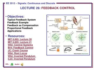
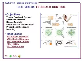
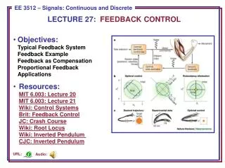
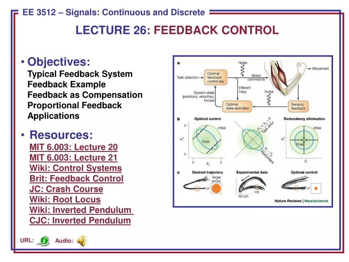
LECTURE 26: FEEDBACK CONTROL. Objectives: Typical Feedback System Feedback Example Feedback as Compensation Proportional Feedback Applications

E N D
LECTURE 26: FEEDBACK CONTROL • Objectives:Typical Feedback SystemFeedback ExampleFeedback as CompensationProportional FeedbackApplications • Resources:MIT 6.003: Lecture 20MIT 6.003: Lecture 21Wiki: Control SystemsBrit: Feedback ControlJC: Crash CourseWiki: Root LocusWiki: Inverted Pendulum CJC: Inverted Pendulum Audio: URL:
A Typical Feedback System Feed Forward Feedback • Why use feedback? • Reducing Nonlinearities • Reducing Sensitivity to Uncertainties and Variability • Stabilizing Unstable Systems • Reducing Effects of Disturbances • Tracking • Shaping System Response Characteristics (bandwidth/speed)
Motivating Example • Open loop system: aim and shoot. • What happens if you miss? • Can you automate the correctionprocess? • Closed-loop system: automatically adjusts until the proper coordinates are achieved. • Issues: speed of adjustment, inertia, momentum, stability, …
System Function For A Closed-Loop System • The transfer function of thissystem can be derived usingprinciples we learned inChapter 6: • Black’s Formula: Closed-loop transfer function is given by: • Forward Gain: total gain of the forward path from the inputto the output, where the gain of a summer is 1. • Loop Gain: total gain along the closed loop shared by all systems. Loop
The Use Of Feedback As Compensation • Assume the open loopgain is very large(e.g., op amp): Independent of P(s) • The closed-loop gain depends only on the passive components (R1 and R2) and is independent of the open-loop gain of the op amp.
Stabilization of an Unstable System • If P(s) is unstable, can westabilize the system byinserting controllers? • Design C(s) and G(s) so thatthe poles of Q(s) are in the LHP: • Example: Proportional Feedback (C(s) = K) • The overall system gain is: • The transfer function is stable for K > 2. • Hence, we can adjust K until the system is stable.
Second-Order Unstable System • Try proportional feedback: • One of the poles is at • Unstable for all values of K. • Try damping, a term proportional to : • This system is stable as long as: • K2 > 0: sufficient damping force • K1 > 4: sufficient gain • Using damping and feedback, we have stabilized a second-order unstable system.
The Concept of a Root Locus • Recall our simple control systemwith transfer function: • The controllers C(s) and G(s) can bedesigned to stabilize the system, but that could involve a multidimensional optimization. Instead, we would like a simpler, more intuitive approach to understand the behavior of this system. • Recall the stability of the system depends on the poles of 1 + C(s)G(s)P(s). • A root locus, in its most general form, is simply a plot of how the poles of our transfer function vary as the parameters of C(s) and G(s) are varied. • The classic root locus problem involves a simplified system: Closed-loop poles are the same.
Example: First-Order System • Consider a simple first-order system: • The pole is at s0 = -(2+K). Vary Kfrom 0 to : • Observation: improper adjustment of the gain can cause the overall system to become unstable. Becomes less stable Becomes more stable
Example: Second-Order System With Proportional Control • Using Black’s Formula: • How does the step responsevary as a function of the gain, K? • Note that as K increases, thesystem goes from too little gainto too much gain.
How Do The Poles Move? Desired Response • Can we generalize this analysis to systems of arbitrary complexity? • Fortunately, MATLAB has support for generation of the root locus: • num = [1]; • den = [1 101 101]; (assuming K = 1) • P = tf(num, den); • rlocus(P);
Summary • Introduced the concept of system control using feedback. • Demonstrated how we can stabilize first-order systems using simple proportional feedback, and second-order systems using damping (derivative proportional feedback). • Why did we not simply cancel the poles? • In real systems we never know the exact locations of the poles. Slight errors in predicting these values can be fatal. • Disturbances between the two systems can cause instability. • There are many ways we can use feedback to control systems including feedback that adapts over time to changes in the system or environment. • Discussed an application of feedback control involving stabilization of an inverted pendulum.
More General Case • Assume no pole/zero cancellation in G(s)H(s): • Closed-loop poles are the roots of: • It is much easier to plot the root locus for high-order polynomials because we can usually determine critical points of the plot from limiting cases(e.g., K= 0, ), and then connect the critical points using some simple rules. • The root locus is defined as traces of s for unity gain: • Some general rules: • At K= 0, G(s0)H(s0) = s0are the poles of G(s)H(s). • At K= , G(s0)H(s0) = 0 s0are the zeroes of G(s)H(s). • Rule #1: start at a pole at K= 0 and end at a zero at K= . • Rule #2: (K 0) number of zeroes and poles to the right of the locus point must be odd.
Inverted Pendulum • Pendulum which has its mass above its pivot point. • It is often implemented with the pivot point mounted on a cart that can move horizontally. • A normal pendulum is stable when hanging downwards, an inverted pendulum is inherently unstable. • Must be actively balanced in order to remain upright, either by applying a torque at the pivot point or by moving the pivot point horizontally (Wiki).
Feedback System – Use Proportional Derivative Control • Equations describing the physics: • The poles of the system are inherentlyunstable. • Feedback control can be used to stabilize both the angle and position. • Other approaches involve oscillatingthe support up and down.