Download
1 / 36
360 likes | 530 Views
XBT Fall Rate Problem A Historical Perspective Bill Emery, Univ. of Colorado Bob Heinmiller (deceased 2005). In the early 1980’s the XBT probes in widest use were: The T4 probe which went to about 500 m and The T7 probe which went to about 700 m.

E N D
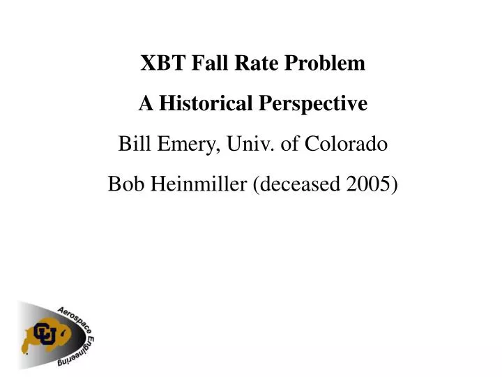
XBT Fall Rate Problem A Historical Perspective Bill Emery, Univ. of Colorado Bob Heinmiller (deceased 2005)
In the early 1980’s the XBT probes in widest use were: The T4 probe which went to about 500 m and The T7 probe which went to about 700 m. The latter become the “deep-blue” probe which has seen the widest use in oceanography. Much of this material is taken from a paper by Bob Heinmiller, Curt Ebbesmeyer, Bruce Taft, Don Olson and Oleg Nikitin published in Deep-Sea Res. in 1983.
This was the era of MODE and POLYMODE so many of these XBT - CTD comparisons were made on US and then USSR research vessels.
Previous Comparisons • As part of the INDOPAC expedition Arnold Mantyla dropped 11 T4 probes with coincident Nansen casts reporting a linear decrease in isotherm depth difference from 0 at the surface to -16 m at 450 m depth. • A series of XBT-CTD comparisons were made in the mid-1970’s (Flierl, 1974; Flierl and Robinson, 1977; McDowell, 1977; Federov et al., 1978 and Seaver and Kuleshov, 1979,82) which all noted systematic differences between T7 XBT and corresponding CTD depths. As shown in table 1 there were a total of 178 comparisons of which 35% were taken at the same time as the CTD profile while the rest were taken half way between the CTD stations.
T4 and T7 comparisons • As part of NORPAX in data set 11 all of the T4 XBT’s were dropped immediately after the CTD profiles. It should be noted that during this time comparisons between CTD temperatures and coincident reversing thermometer data yielded a mean difference of 0.006 °C and a standard deviation of 0.02 °C which should be taken as an upper limit on the accuracy of the CTD temperature measurements. • Between 1976 and 1978 data sets 12-15 were collected using T7 probes dropped during or immediately after a Niel-Brown CTD cast. In most of these profiles coincident reversing thermometers were used to provide corrections for the CTD temperatures (Iselin 0.0026 °C, Gyre 0.0034 °C)
10 of the 15 available data sets were edited as follows: • for data sets 6 to 11 the 2 CTD temperature profiles adjacent to the XBT temperature were linearly interpolated to the position of the XBTcast. • Means and standard deviations were computed for the T4 XBT - CTD temperatures (data sets 6 - 11) and for the T7 XBT - CTD (data sets 12 - 15).
• A T4 XBT profile was rejected if at any depth the temperature difference with the CTD profile exceeded 3 times the standard deviation (again only for data sets 6 - 11). This resulted in a rejection of about 8 - 16% of the XBT profiles. • A T7 XBT profile was rejected if this same difference exceeded 1.5 X standard deviation which resulted in a rejected of about 18 - 21 % of the XBT temperature profiles being eliminated.
• This analysis is based on the assumption that we can have both systematic errors that are independent of depth and depth dependent errors. • Sources of the systematic errors are temperature offsets due to incorrect balancing of the thermistor (see next slides), incorrect weight of the probe (next slides), etc. • Sources of the latter are the changing mass with the outlay of copper wire, the changing water density and hence friction, etc.
• To account for temperature errors the profiles were first examined in regions where the vertical temperature gradients were very small (thermostads) and the XBT profiles were corrected for any offsets observed in these layers before the depth dependent errors were calculated.
• Thermostads were found in the 50 m mixed layer (T4’s in 6-11), in the 125 m mixed layer near a Gulf Stream ring (T7; 12) and in the 18°C water (T7; 13-15). • The mean temperature gradient in the 25 m Pacific mixed layer was taken to be ≥-0.01 °C/m (sets 6-11) which in the North Atlantic thermostads was ≥-0.006 °C/m. • Previous studies suggested that XBT depth errors in the thermostads were about 3 m resulting in a temperature error of -0.03 which about half of the 0.05 °C resolution possible with an XBT profile.
• Since this is much smaller than the mean temperature differences between the XBT and CTD in Table 3 we conclude that we don’t need to include the depth-dependent error in the thermostads and we can use them for temperature “calibration.” • Georgi et al. (1980) carefully calibrated XBT probes in a constant thermal bath and found that temperature errors varied between -0.011 and 0.014 °C over a range of 0 to 30 °C. • These differences are small relative to the 0.17 °C mean temperature difference in Table 3 which means that the XBT temperature errors are not significant in calculating the depth errors.
• Returning to Table 3 we note that for data set 11 the XBT and CTD casts were nearly coincident and that the s.d. of 0.18 °C is close to the mean s.d. of 0.23 °C. • This mean s.d. is twice as large as that for the T7 probes. • Thus, we conclude that this variability is characteristic of these two types of XBT probes.
• After all the XBT profiles were adjusted for the thermostad “calibration” differences in XBT and CTD isotherm depths (dz) were computed along with the mean difference ( ) and the standard deviation of the differences (sdz). • Note: depth values were linearly interpolated for sets 2, 4 and 5, 6 m was subtracted from depths given by Seaver and Kuleshov to correct for the offset reported, Federov et al. reported depth differences only as a function of temperature so data set 3 was not considered in the comparisons, and a reported correction of 8 m was added to data set 12.
• Both T4 and T7 difference profiles start positive near the surface and then turn negative. This inflection point is at 150 m for the T4’s and 400 m for the T7’s. • In general the T4’s have larger differences beneath the inflection point and also show larger variability between the different data sets. • We now turn to the standard deviations of these differences which show a surprising similarity for all of the T4 data sets and some very marked variability in the upper 400 m of the T7 profiles.
• Note data sets 6 - 10 were those T4 profiles separated by 30 km while in data set 11 the XBT and CTD profiles were nearly coincident. • Thus, while the 6-10 profiles show a similar but increasing variability with depth data set 11 shows a rapid decrease from the surface down to 100 m below which the variability is nearly constant at 10 m. • A very similar variability limit of about 10 m is seen for the T7 profiles in data set 12 which was close to a Gulf Stream ring. • Data sets 13-15 were collected from Feb. to July, 1978 in the area of the 18 °C mode water. • It is the presence of the mode water in these profiles that causes the large variations in depth difference in the upper layers not the performance of the XBT probes.
• Below the 18 °C mode water the T7 XBT depth difference variability is nearly constant again at about 10 m. • This suggests that the error is not depth-dependent and has a mean value of 10 m for both types of XBT probes. • To test this conclusion statistically we carried out an F-test analysis of our results. • We used for our F-test where m is the number of data sets, n is the number in data set i, is the mean of data set i, si is the standard deviation of xi, is the equally weighted overall mean of the data .
• We have modified the F-test to use only means and standard deviations and to apply the test to data sets of differing size. • To apply the tests the depth differences in Table 1 were interpolated to common depths at 25 m (T4 probes) and 125 m (T7 probes) intervals. • For the T4 probes the F-test results exceeded the 5% critical level for most depths, which indicated that the six mean curves are not homogeneous. • For the T7 probes the F-test indicates that all depths except between 150 and 250 m the mean values of depth differences were statistically similar at the 5% critical level.
• Because of the F-test results we determined that we could not develop a correction for the T4 profiles and thus concentrated only on the T7 data. • The next figure is a plot of the T7 mean differences obtained by averaging the T7 profiles in Fig. 2b. • Each data set was equally weighted. • We also include the dotted lines shown in Fig. 2 which can be used to represent different portions of the T7 profiles.
• This figure suggests that the differences can be approximated by 2 straights line segments. • So we fitted the data in the following table to two straight line segments using a least-squares fit. • The resulting equations are: Where zx is the XBT depth and zc is the CTD depth in meters.
• The maximum deviation from this linear fit is 1.9 at 550 m depth. • The RMS deviation from the curve fit is 0.75 m. • The mean deviations are in general < 1/10 of the standard deviations of the differences. • We conclude that the linear fits are a good approximations to the depth differences. • Attempts to use other difference formulations resulted in larger RMS differences.
• In these equations XBT depth is defined in terms of the CTD depth which is not known. • For practical use the CTD depth should be expressed in terms of the XBT depth as: Only for T7 probes.
• It should be emphasized that this analysis was based on older analog XBT data which suffers from additional recording errors not found in modern digital systems. • This in part was our motivation for the termostad “calibration.” • We also note that while the given precision of the XBT even in these older systems was given as 0.1 °C but our comparisons demonstrated T7 mean differences of 0.19 °C with a standard deviation of 0.11 °C.