Download
1 / 9
100 likes | 371 Views
Complex Waveforms as Input. When complex waveforms are used as inputs to the circuit (for example, as a voltage source), then we (1) must Laplace transform the inputs (2) determine the transfer function (3) feed the input through the transfer function

E N D
Complex Waveforms as Input • When complex waveforms are used as inputs to the circuit (for example, as a voltage source), then we (1) must Laplace transform the inputs (2) determine the transfer function (3) feed the input through the transfer function • The transfer function, H(s), is the ratio of some output variable to some input variable Lecture 19
Transfer Function • The transfer function, H(s), is • All initial conditions are zero (makes transformation step easy) • Can use transfer function to find output to an arbitrary input Y(s) = H(s) X(s) • The impulse response is the inverse Laplace transform of transfer function h(t) = L-1[H(s)] with knowledge of the transfer function or impulse response, we can find response of circuit to any input Lecture 19
Variable-Frequency Response Analysis • As an extension of ac analysis, we now vary the frequency and observe the circuit behavior • Graphical display of frequency dependent circuit behavior can be very useful; however, quantities such as the impedance are complex valued such that we will tend to graph the magnitude of the impedance versus frequency (i.e., |Z(j)| v. f) and the phase angle versus frequency (i.e., Z(j) v. f) Lecture 19
Frequency Response of a Resistor • Consider the frequency dependent impedance of the resistor, inductor and capacitor circuit elements • Resistor (R): ZR = R 0° So the magnitude and phase angle of the resistor impedance are constant, such that plotting them versus frequency yields R Magnitude of ZR () Phase of ZR (°) 0° Frequency Frequency Lecture 19
Frequency Response of an Inductor • Inductor (L): ZL = L 90° The phase angle of the inductor impedance is a constant 90°, but the magnitude of the inductor impedance is directly proportional to the frequency. Plotting them vs. frequency yields (note that the inductor appears as a short at dc) 90° Magnitude of ZL () Phase of ZL (°) Frequency Frequency Lecture 19
Frequency Response of a Capacitor • Capacitor (C): ZC = 1/(C)–90° The phase angle of the capacitor impedance is –90°, but the magnitude of the inductor impedance is inversely proportional to the frequency. Plotting both vs. frequency yields (note that the capacitor acts as an open circuit at dc) Magnitude of ZC () Phase of ZC (°) -90° Frequency Frequency Lecture 19
X(j)ejt = X(s)est Y(j)ejt = Y(s)est H(j) = H(s) Transfer Function • Recall that the transfer function, H(s), is • The transfer function can be shown in a block diagram as • The transfer function can be separated into magnitude and phase angle information, H(j) = |H(j)| H(j) Lecture 19
Common Transfer Functions • Since the transfer function, H(j), is the ratio of some output variable to some input variable, • We may define any number of transfer functions • ratio of output voltage to input current, i.e., transimpedance, Z(jω) • ratio of output current to input voltage, i.e., transadmittance, Y(jω) • ratio of output voltage to input voltage, i.e., voltage gain, GV(jω) • ratio of output current to input current, i.e., current gain, GI(jω) Lecture 19
Poles and Zeros • The transfer function is a ratio of polynomials • The roots of the numerator, N(s), are called the zeros since they cause the transfer function H(s) to become zero, i.e., H(zi)=0 • The roots of the denominator, D(s), are called the poles and they cause the transfer function H(s) to become infinity, i.e., H(pi)= Lecture 19