Download

1 / 133
1.33k likes | 1.33k Views
07/12/2011. ArcGIS Server Performance and Scalability—Testing Methodologies. Andrew Sakowicz Frank Pizzi. Introductions. Who are we? Enterprise implementation Target audience GIS administrators DBAs Architects Developers Project managers Level Intermediate. Objectives.

E N D
07/12/2011 ArcGIS Server Performance and Scalability—Testing Methodologies Andrew Sakowicz Frank Pizzi
Introductions • Who are we? • Enterprise implementation • Target audience • GIS administrators • DBAs • Architects • Developers • Project managers • Level • Intermediate
Objectives Performance engineering—concepts and best practices • Technical • Solution performance factors • Tuning techniques • Performance testing • Capacity planning • Managerial • Skills • Level of effort • Risks • ROI
Agenda Solution performance engineering • Introduction • Performance engineering in project phases • Requirements • Design Lunch • Development • Deployment • Operation and maintenance
Performance Engineering Benefits • Lower costs • Optimal resource utilization • Less hardware and licenses • Higher scalability • Higher user productivity • Better performance • Reputation • User satisfaction
Performance and Scalability Definitions • Performance: The speed at which a given operation occurs • Scalability: The ability to maintain performance as load increases
Performance and Scalability Definitions Throughput: The amount of work accomplished by the system in a given period of time
Performance and Scalability Definitions Defining system capacity • System capacity can be defined as a user load corresponding to • Maximum throughput • Threshold utilization, e.g., 80 • SLA response time
Project Life Cycle Phase Performance engineering applied at each step
Project Life Cycle Phase Performance engineering applied at each step • Requirements • Quality attributes, e.g., SLA • Design • Performance factors, best practices, capacity planning • Development • Performance and load testing • Tuning • Deployment • Configuration, tuning, performance, and load testing • Operation and maintenance • Tuning • Capacity validation
Requirements Phase Performance engineering addresses quality attributes. • Quality Attribute Requirements Functional Requirements • Visualization • Analysis • Workflow Integration • Availability • Performance & Scalability • Security
Requirements Phase • Define System Functions • What are the functions that must be provided? • Define System Attributes • Nonfunctional requirements should be explicitly defined. • Risk Analysis • An assessment of requirements • Intervention step designed to prevent project failure • Analyze/Profile Similar Systems • Design patterns • Performance ranges
Design Phase Selection of optimal technologies • Meet functional and quality attributes. • Consider costs and risks. • Understand technology tradeoffs, e.g.: • Application patterns • Infrastructure constraints • Virtualization • Centralized vs. federated architecture
Design Phase Performance Factors
Design Phase—Performance Factors Design, Configuration, Tuning, Testing • Application • GIS Services • Hardware Resources
Design Phase—Performance Factors Application • Type, e.g., mobile, web, desktop • Stateless vs. state full (ADF) • Design • Chattiness • Data access (feature service vs. map service) • Output image format
Design Phase—Performance Factors Application Types • Architecture • resources.arcgis.com/content/enterprisegis/10.0/architecture
Design Phase—Performance Factors Application Security • Security • resources.arcgis.com/content/enterprisegis/10.0/application_security
Design Phase—Performance Services Application—Output image format • PNG8/24/32 • Transparency support • 24/32 good for antialiasing, rasters with many colors • Lossless: Larger files ( > disk space/bandwidth, longer downloads) • JPEG • Basemap layers (no transparency support) • Much smaller files
Design Phase—Performance Factors GIS Services
Design Phase—Performance Factors GIS Services—Map Service Source document (MXD) optimizations • Keep map symbols simple. • Avoid multilayer, calculation-dependent symbols. • Spatial index. • Avoid reprojections on the fly. • Optimize map text and labels for performance. • Use annotations. • Cost for Maplex and antialiasing. • Use fast joins (no cross db joins). • Avoid wavelet compression-based raster types (MrSid, JPEG2000).
Design Phase—Performance Factors GIS Services—Map service • Performance linearly related to number of features
Design Phase—Performance Factors Performance Test Cache vs. MSD vs. MXD When possible, use Optimized Services for dynamic data. Single user response times are similar. If data is static, use cache map Services. Cache map services use the least of hardware resources.
Design Phase—Performance Factors GIS Services—Geoprocessing • Precompute intermediate steps when possible. • Use local paths to data and resources. • Avoid unneeded coordinate transformations. • Add attribute indexes. • Simplify data.
Design Phase—Performance Factors GIS Services—GP vs. Geometry Single user response times are similar. Use geometry service for simple operations such as buffering and spatial selections.
Design Phase—Performance Factors GIS Services—Image • Tiled, JPEG compressed TIFF is the best (10–400% faster). • Build pyramids for raster datasets and overviews for mosaic datasets. • Tune mosaic dataset spatial index. • Use JPGPNG request format in web and desktop clients. • Returns JPEG unless there are transparent pixels (best of both worlds).
Design Phase—Performance Factors GIS Services—Geocode • Use local instead of UNC locator files. • Services with large locators take a few minutes to warm up. • New 10 Single Line Locators offer simplicity in address queries but might be slower than traditional point locators.
Design Phase—Performance Factors GIS Services—Geocode Line Single user response times are similar. Point
Design Phase—Performance Factors GIS Services—Geodata • Database Maintenance/Design • Keep versioning tree small, compress, schedule synchronizations, rebuild indexes and have a well-defined data model. • Geodata Service Configuration • Server Object usage timeout (set larger than 10 min. default) • Upload/Download default IIS size limits (200 K upload/4 MB download)
Design Phase—Performance Factors GIS Services—Feature • Trade-off between client-side rendering and sending large amounts of data over the wire
Design Phase—Performance Factors GIS Services—Data storage • Typically a low impact • Small fraction (< 20%) of total response time
Design Phase—Performance Factors GIS Services—Data source location • Local to SOC machine • UNC (protocol + network latency overhead) All disks being equal, locally sourced data results in better throughput.
Design Phase—Performance Factors GIS Services—ArcSOC instances ArcSOC Instances max = n * #CPU Cores n = 1 … 4 If max SOC instances are underconfigured, system will not scale.
Design Phase—Capacity Planning CPU Factors • User load: Concurrent users or throughput • Operation CPU service time (model)—performance • CPU SpecRate subscript t = target subscript b = benchmark ST = CPU service time TH = throughput %CPU = percent CPU
Design Phase—Capacity Planning • Service time determined using a load test • Capacity model expressed as Service Time
Design Phase—Capacity Planning Additional Resources • System Designer • Guide: Capacity Planning and Performance Benchmarks • resources.arcgis.com/gallery/file/enterprise-gis/details?entryID=6367F821-1422-2418-886F-FCC43C8C8E22 • CPT • http://www.wiki.gis.com/wiki/index.php/Capacity_Planning_Tool
Design Phase—Capacity Planning Uncertainty of input information—Planning hour • Identify the Peak Planning Hour (most cases)
Design Phase—Capacity Planning Uncertainty of input information High Low Define user load first
Design Phase—Capacity Planning Uncertainty of input information • License • Total employees • Usage logs
Design Phase—Performance Factors Hardware Resources
Design Phase—Performance Factors Hardware Resources • CPU • Network bandwidth and latency • Memory • Disk Most well-configured and tuned GIS systems are processor-bound.
Design Phase—Performance Factors Hardware Resources—Virtualization overhead
Design Phase—Performance Factors Hardware Resources—Network bandwidth directionality
Design Phase—Performance Factors Hardware Resources—Network • Distance • Payload • Infrastructure
Design Phase—Performance Factors Hardware Resources—Network