Download
1 / 14
190 likes | 475 Views
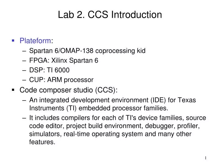
Lab 2. CCS Introduction Plateform : Spartan 6/OMAP-138 coprocessing kid FPGA: Xilinx Spartan 6 DSP: TI 6000 CUP: ARM processor Code composer studio (CCS): An integrated development environment (IDE) for Texas Instruments (TI) embedded processor families.

E N D
Lab 2. CCS Introduction • Plateform: • Spartan 6/OMAP-138 coprocessing kid • FPGA: Xilinx Spartan 6 • DSP: TI 6000 • CUP: ARM processor • Code composer studio (CCS): • An integrated development environment (IDE) for Texas Instruments (TI) embedded processor families. • It includes compilers for each of TI's device families, source code editor, project build environment, debugger, profiler, simulators, real-time operating system and many other features.
The plateform: Power On/off Ethernet plug USB plug S7 switch Reset
The setting of S7 switch: • The first, the fifth, and the eighth switches must be on (DSP only). • The other setting is that all are off except the first one (DSP and ARM). • Turn on the plateform.
Activate the CCS form the Program files • TI Code composer studio v5 • First, you have select a directory for the workspace. • Then, File New create a CCS project. • Give a project name and select the family of the device as C6000, and the variant as OMP138.
Click the finish icon and you are ready to edit a C file. • After you finish the editing, you can select • Proj Built all • Make sure you are in the Edit mode rather than Debug mode (shown on the right up corner). • Then, click • Run Debug (link/loading) • If there is an error indicating the system is in reset, then press Reset and try again. • If there is an error indicating a target configuration is needed, press “yes” and • Select the device TI XDS100v2 USB emulator, • Then press “save”. * Print a couple of words.
Finally, you can click Run Resume to execute the program. • If you want to execute the program again, you can click Run Restart • Once the program has been executed, you can click the Terminate to return the edit mode.
Icons: Resume Terminate Pause
Make sure to include stdio header file (#include <stdio.h>) • Practice 1: • Run the convolution program created in the last week in the CCS environment. • In CCS, you can plot the signal stored in the memory. • Must in the pause mode (put an idle loop). • Debug Run Pause • Tools graphic single time • Change the parameters for the plot * for (; ;) { }
Then, length data type decimation factor signal display length
You can also plot the spectrum of a signal. • Tools graph FFT magnitude interlaced input Complex FFT size: 2n Graph properties: re-input parameters
CCS provides many build-in routines in its libraries. Before they can be used, we have to do some setup. • Select Project and then Properties: • Properties C6000 compiler include options • Add one option: “C:\Program Files\Texas Instruments\dsplib_c674x_3_1_0_0\packages\” (in the upper blank) • Properties C6000 linker file search path • Add one file: “C:\Program Files\Texas Instruments\dsplib_c674x_3_1_0_0\lib/dsplib.a674” (in the upper blank) • Copy dsplib.h into the project you are working on and add “ #include “dsplib.h” ” in your C program.
Use the convolution routine from the DSP library: • DSPF_sp_convol(x, h, y, nh, ny); • x: input signal, h: filter, y: output signal • nh: length of h, ny: length of y (both have to be even) • x has to be zero padded (before and after x) • If there are more than one C programs in a project. You can de-activate one by pressing right mouse on the file and selecting Recourse configuration and then Exclude from Build ... (check Debug and Release) • Practice 2: • Use the build-in routine to conduct the convolution operation and compare the result with the one you have written.
Use the FFT routine from the DSP library: • DSPF_sp_fftSPxSP(N, x, w, y, brev, n_min, offset, n_max) • N: the size of FFT (N=2m) • x, y: input/output (even: real, old: imaginary) with length 2N • brev: unsign characters with 64 entries (defined globally) • w: generated by another function gen_twiddle_fft_sp(w,N) • n_min: 2 or 4 (N=2m; and m is divided by 2 or 4; choose the larger one) • offset: index from the start of main FFT (typical 0) • n_max: N • Practice 3: • Use the build-in routine to see the spectrum of the signals generated in Practice 2. * After the calling, the input values may be changed (must be defined as global var. for plotting)
Reading assignment: • Digital modulation: PAM, QAM (CS: 6.1-6.4) • AWGN • Error probability (Q-function) * Textbooks: CS: Communication System S&S: Signals and Systems