In summary

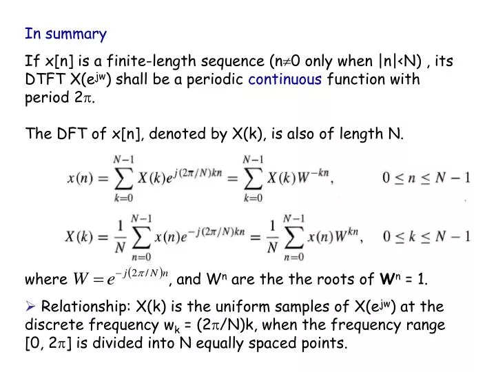
1. In summary If x[n] is a finite-length sequence (n0 only when |n|<N) , its DTFT X(ejw) shall be a periodic continuous function with period 2. The DFT of x[n], denoted by X(k), is also of length N. where , and Wn are the the roots of Wn = 1. • Relationship: X(k) is the uniform samples of X(ejw) at the discrete frequency wk = (2/N)k, when the frequency range [0, 2] is divided into N equally spaced points.

2. x[n] T{} y[n] The Concept of ‘System’ (oppenheim et al. 1999) • Discrete-time Systems • A transformation or operator that maps an input sequence with values x[n] into anoutput sequence with value y[n] . y[n] = T{x[n]}

3. System Examples • Ideal Delay • y[n] = x[nnd], wherendis a fixed positive integer called the delay of the system. • Moving Average • Memoryless Systems • The output y[n] at every value of n depends only on the input x[n], at the same value of n. • Eg. y[n] = (x[n])2, for each value of n.

4. System Examples (continue) • Linear System: If y1[n] and y2[n] are the responses of a system when x1[n] and x2[n] are the respective inputs. The system is linear if and only if • T{x1[n] + x2[n]} = T{x1[n] }+ T{x2[n]} = y1[n] + y2[n] . • T{ax[n] } = aT{x[n]} = ay[n], for arbitrary constant a. • So, if x[n] = k akxk[n], y[n] = k akyk[n] (superposition principle) • For example Accumulator System (is a linear system)

5. System Examples (continue) • Nonlinear System. • Eg. w[n] = log10(|x[n]|) is not linear. • Time-invariant System: • If y[n] = T{x[n]}, then y[nn0] = T{x[n n0]} • The accumulator is a time-invariant system. • The compressor system (not time-invariant) • y[n] = x[Mn],  < n < .

6. System Examples (continue) • Causality • A system is causal if, for every choice of n0, the output sequence value at the index n =n0 depends only the input sequence values for n n0. • That is, if x1[n] = x2[n] forn n0, then y1[n] = y2[n] forn n0. • Eg. Forward-difference system (non causal) • y[n] = x[n+1]  x[n] (The current value of the output depends on a future value of the input) • Eg. Background-difference (causal) • y[n] = x[n]  x[n1]

7. System Examples (continue) • Stability • Bounded input, bounded output (BIBO): If the input is bounded, |x[n]|  Bx <  for all n, then the output is also bounded, i.e., there exists a positive value By s.t. |y[n]|  By <  for all n. • Eg., the system y[n] = (x[n])2is stable. • Eg., the accumulated system is unstable, which can be easily verified by setting x[n] = u[n], the unit step signal.

8. Linear Time Invariant Systems • A system that is both linear and time invariant is called a linear time invariant (LTI) system. • By setting the input x[n] as [n], the impulse function, the output h[n] of an LTI system is called the impulse response of this system. • Time invariant: when the input is [n-k], the output is h[n-k]. • Remember that the x[n] can be represented as a linear combination of delayed impulses

9. Linear Time Invariant Systems (continue) • Hence • Therefore, a LTI system is completely characterized by its impulse response h[n].

10. Linear Time Invariant Systems (continue) • Note that the above operation is convolution, and can be written in short by y[n] = x[n]  h[n]. • The output of an LTI system is equivalent to the convolution of the input and the impulse response. • In a LTI system, the input sample at n = k, represented as x[k][n-k], is transformed by the system into an output sequence x[k]h[n-k] for  < n < .

11. h1[n] h2[n] h2[n] h1[n] x[n] x[n] y[n] y[n] h1[n]  h2[n] y[n] x[n] Property of LTI System and Convolution • Communitive • x[n]  h[n] = h[n]  x[n]. • Distributive over addition • x[n]  (h1[n] + h2[n]) = x[n]  h1[n] + x[n] h2[n]. • Cascade connection

12. Property of LTI System and Convolution (continue) • Parallel combination of LTI systems and its equivalent system.

13. Property of LTI System and Convolution (continue) • Stability: A LTI system is stable if and only if Since when |x[n]|  Bx. • This is a sufficient condition proof.

14. Property of LTI System and Convolution (continue) • Causality • those systems for which the output depends only on the input samples y[n0] depends only the input sequence values for n n0. • Follow this property, an LTI system is causal iff h[n] = 0 for all n <0. • Causal sequence: a sequence that is zero for n<0. A causal sequence could be the impulse response of a causal system.

15. Impulse Responses of Some LTI Systems • Ideal delay: h[n] = [n-nd] • Moving average • Accumulator • Forward difference: h[n] = [n+1][n] • Backward difference: h[n] = [n][n1]

16. Examples of Stable/Unstable Systems • In the above, moving average, forward difference and backward difference are stable systems, since the impulse response has only a finite number of terms. • Such systems are called finite-duration impulse response (FIR) systems. • FIR is equivalent to a weighted average of a sliding window. • FIR systems will always be stable. • The accumulator is unstable since

17. Examples of Stable/Unstable Systems (continue) • When the impulse response is infinite in duration, the system is referred to as an infinite-duration impulse response (IIR) system. • The accumulator is an IIR system. • Another example of IIR system: h[n] = anu[n] • When |a|<1, this system is stable since S = 1 +|a| +|a|2 +…+ |a|n+…… =1/(1|a|) is bounded. • When |a| 1, this system is unstable

18. Examples of Causal Systems • The ideal delay, accumulator, and backward difference systems are causal. • The forward difference system is noncausal. • The moving average system is causal requires M10 and M20.

19. Equivalent Systems • A LTI system can be realized in different ways by separating it into different subsystems.

20. Equivalent Systems (continue) • Another example of cascade systems – inverse system.

21. Linear Constant-coefficient Difference Equations for alln • An important subclass of LTI systems consist of those system for which the input x[n] and output y[n] satisfy an Nth-order linear constant-coefficient difference equation. • A general form is shown above. • Not-all LTI systems can be represented into this form, but it specifies a wide class of LTI systems.

22. + + + + + + + + x[n] y[n] b0 TD TD TD TD TD TD bM b2 b1  a2  aN  a1 y[n-1] x[n-1] x[n-2] y[n-2] y[n-N] x[n-M] Block Diagram of the Difference Equation • Assume that a0 = 1. Let TD denote one-sample delay.

23. Difference Equation: FIR system • The assumption a0 = 1 can be always achieved by dividing all the coefficients by a0if a00. • The difference equation characterizes a recursive way of obtaining the output y[n] from the input x[n]. • When ak = 0 for k = 1 … N, the difference equation degenerates to a FIR (finite impulse response) system - the impulse response is of finite length. • The output consists of a linear combination of finite inputs.

24. Difference equation: IIR System • When bmare not all zerosfor m = 1 … M, and a0 = 1, the difference equation degenerates to • This is an example of IIR (infinite impulse response) system • IIR system: systems with the the impulse response being of infinite length.

25. Example • Accumulator

26. Example (continue) • Moving average system when M1=0: • The impulse response is h[n] = u[n]  u[nM2 1] • Also, note that The term y[n]  y[n1] suggests the implementation can be cascaded with an accumulator.

27. + + + + b TD TD TD x[n] y[n] b b b x[n-1] x[n-2] x[n-M] Moving Average System • Hence, there are at least two difference equation representations of the moving average system. First, where b = 1/ (M2+1) and TD denotes one-sample delay

28. Moving Average System (continue) • Second, • The first representation is FIR, and the second is IIR.

29. Solution of Difference Equations • Just as differential equations for continuous-time systems, a linear constant-coefficient difference equation for discrete-time systems does not provide a unique solution if no additional constraints are provided. • Solution: y[n] = yp[n] + yh[n] • yh[n]: homogeneous solution obtained by setting all the inputs as zeros. • yh[n]: a particular solution satisfying the difference equation.

30. Solution of Difference Equations (continue) • Additional constraints: consider the N auxiliary conditions that y[1], y[2], …, y[N] are given. • The other values of y[n] (n0) can be generated by when x[n] is available, y[1], y[2], … y[n], … can be computed recursively. • To generate values of y[n] for n<N recursively,

31. Example of the Solutions • Consider the difference equation y[n] = ay[n-1] + x[n]. • Assume the input is x[n] =K  [n], and the auxiliary condition is y[1] = c. • Hence, y[0] = ac+K, y[1] = a y[0]+0 = a2c+aK, … • Recursively, we found that y[n] = an+1c+anK, forn0. • For n<1, y[-2] = a1(y[1]x[1] ) = a1c, y[2] = a1 y[1] = a2 c, …, and y[n] = an+1c for n<1. • Hence, the solution is y[n] = an+1c+Kanu[n],

32. Example of the Solutions (continue) • The solution system is non-linear: • When K=0, i.e., the input is zero, the solution (system response) y[n] = an+1c. • Since a linear system requires that the output is zero for all time when the input is zero for all time. • The solution system is not shift invariant: • when input were shifted by n0 samples, x1[n] =K  [n - n0], the output is y1[n] = an+1c+Kann0u[n - n0]. • The recursively-implemented system for finding the solution is non-causal.

33. LTI solution of difference equations • Our principal interest in the text is in systems that are linear and time invariant. • How to make the recursively-implemented solution system be LTI? • Initial-rest condition: • If the input x[n] is zero for n less than some time n0, the output y[n] is also zero for n less than n0. • The previous example does not satisfy this condition since x[n]= 0 for n<0 but y[1] = c. • Property: If the initial-rest condition is satisfied, then the system will be LTI and causal.

34. Frequency-Domain Representation of Discrete-time Signals and Systems • Eigen function of a LTI system • When applying an eigenfunction as input, the output is the same function multiplied by a constant. • x[n] = ejwn is the eigenfunction of all LTI systems. • Let h[n] be the impulse response of an LTI system, when ejwn is applied as the input,

35. Eigenfunction of LTI • Let we have • Consequently, ejwn is the eigenfunction of the system, and the associated eigenvalue is H(ejw). • Remember that H(ejw) is the DTFT of h[n] . • We call H(ejw) the LTI system’s frequency response • consisting of the real and imaginary parts, H(ejw)=HR(ejw)+jHI(ejw), or in terms of magnitude and phase.

36. Example of Frequency Response • Frequency response of the ideal delay system, y[n] =x[n  nd], • If we consider x[n] = ejwn as input, then Hence, the frequency response is • The magnitude and phase are

37. Linear Combination • When a signal can be represented as a linear combination of complex exponentials (Fourier Series): By the principle of superposition, the output is • Thus, we can find the output of linearly combined signals if we know the frequency response of the system.

38. Example of Linear Combination • Sinusoidal responses of LTI systems: • The response of x1[n] and x2[n] are • If h[n] is real, by the DTFT property that H(ejw0) = H*(ejw0), the total response y[n]=y1[n]+ y2[n] is

39. Difference to Continuous-time System Response • For a continuous-time system, the frequency response applied is the continuous Fourier transform, which is not necessarily to be periodic. • However, for a discrete-time system, the frequency response is always periodic with period 2, since • Because H(ejw) is periodic with period 2, we need only specify H(ejw) over an interval of length 2, eg., [0,2] or [,]. For consistency, we choose the interval [,]. • The inherent periodicity defines the frequency response everywhere outside the chosen interval.

40. Convolution vs. Multiplication • For DTFT, when performing convolution in time domain, it is equivalent to perform multiplication in the frequency domain. • Hence, for an LTI system with the impulse response being h[n], when the input is x[n] • We know that y[n] = h[n]x[n]. • The spectrum of y[n] shall be Y(ejw) = H(ejw)X(ejw). • i.e., the spectrum of y[n] can be obtained by multiplying the spectrum of x[n] with the frequency response.

41. Ideal Frequency-selective Filters • The “low frequencies” are frequencies close to zero, while the “high frequencies” are those close to . • Since that the frequencies differing by an integer multiple of 2 are indistinguishable, the “low frequency” are those that are close to an even multiple of , while the “high frequencies” are those close to an odd multiple of . • Ideal frequency-selective filters: • An important class of linear-invariant systems includes those systems for which the frequency response is unity over a certain range of frequencies and is zero at the remaining frequencies.

42. Frequency Response of Ideal Low-pass Filter

43. Frequency Response of Ideal High-pass Filter

44. Frequency Response of Ideal Band-stop Filter

45. Frequency Response of Ideal Band-pass Filter

46. Frequency Response of the Moving-average System • The impulse response of the moving-average system is • Therefore, the frequency response is • By noting that the following formula holds:

47. Frequency Response of the Moving-average System (continue) (magnitude and phase)

48. Frequency Response of the Moving-average System (continue) M1= 0 and M2 = 4 Amplitude response Phase response 2w

49. Example • Determining the impulse response for a difference equation y[n](1/2) y[n1] = x[n] (1/4)x[n1] To find the impulse response, we set x[n] = [n]. Then the above equation becomes h[n](1/2) h[n1] = [n]  (1/4)[n1] Applying the Fourier transform, we obtain H(ejw)  (1/2)e-jwH(ejw) = 1  (1/4) e-jw So H(ejw) = (1  (1/4) e-jw) / (1  (1/2) e-jw)

50. Example (continue) • To obtain the impulse response h[n] • From the DTFT pair-wise table, we know that thus, (1/2)nu[n]  1 / (1  (1/2) e-jw) By the shifting property, (1/4)(1/2)n1u[n1]  (1/4) e-jw / (1  (1/2) e-jw) Thus, h[n] = (1/2)nu[n]  (1/4)(1/2)n1u[n1]