Download

1 / 42
420 likes | 639 Views
Lecture 5-6 Object Detection – Boosting. Tae- Kyun Kim. Face Detection Demo. Multiclass object detection [ Torralba et al PAMI 07]. A boosting algorithm, originally for binary class problems, has been extended to multi-class problems. Object Detection.

E N D
Lecture 5-6Object Detection – Boosting Tae-Kyun Kim
Multiclass object detection[Torralbaet al PAMI 07] A boosting algorithm, originally for binary class problems, has been extended to multi-class problems.
Object Detection Input: A single image is given as input, without any prior knowledge.
Object Detection Output is a set of tight bounding boxes (positions and scales) of instances of a target object class (e.g. pedestrian).
Object Detection Scanning windows: We scan every scale and every pixel location in an image.
Number of Hypotheses It ends up with a huge number of candidate windows . x … # of scales # of pixels Number of Windows: e.g.747,666
Time per window What amount of time is given to process a single scanning window? SIFT or raw pixels … …… dimension D Num of feature vectors: 747,666 Classification:
Time per window or raw pixels … …… dimension D Num of feature vectors: 747,666 In order to finish the task say in 1 sec Time per window (or vector): 0.00000134 sec Neural Network? Nonlinear SVM?
Examples of face detection From Viola, Jones, 2001
More traditionally…The search space is narrowed down. • By Integrating Visual Cues [Darrell et al IJCV 00]. • Face pattern detection output (left). • Connected components recovered from stereorange data (mid). • Regions from skin colour (hue) classification (right).
Since about 2001 (Viola &Jones 01)… “BoostingSimple Features” has been a dominating art. • Adaboost classification • Weak classifiers: Haar-basis features/functions • The feature pool size is e.g. 45,396 (>>T) Strong classifier Weak classifier
Introduction to Boosting Classifiers- AdaBoost (Adaptive Boosting)
Boosting • Boosting gives good results even if the base classifiers have a performance slightly better than random guessing. • Hence, the base classifiers are called weakclassifiers or weaklearners.
Boosting For a two (binary)-class classification problem, we train with training data x1,…,xN target variables t1,…,tN, where tN∈ {-1,1}, data weight w1,…,wN weak (base) classifier candidates y(x) ∈ {-1, 1}.
Boosting does Iteratively, 1) reweighting training samples, • by assigning higher weights to previously misclassified samples, 2) finding the best weakclassifier for the weighted samples. 50 rounds 2 rounds 3 rounds 4 rounds 5 rounds 1 round
In the previous example, the weaklearner was defined by a horizontal or vertical line, and its direction. -1 +1
AdaBoost(adaptive boosting) 1. Initialisethe data weights {wn} by wn(1) = 1/N for n = 1,… ,N. 2. For m = 1, … ,M : the number of weak classifiers to choose (a) Learn a classifier ym(x)that minimises the weighted error, among all weak classifier candidates where I is the impulse function. (b) Evaluate
and set (c) Update the data weights 3. Make predictions using the final model by
Minimising Exponential Error • AdaBoost is the sequential minimisationof the exponential error function where tn∈ {-1, 1} and fm(x) is a classifier as a linear combination of base classifiers yl(x) • We minimiseEwith respect to the weight αland the parameters of the base classifiers yl(x).
Sequential Minimisation: suppose that the base classifiers y1(x) ,. …, ym-1(x) and their coefficients α1, …, αm-1are fixed, and we minimise only w.r.t. am and ym(x). • The error function is rewritten by where wn(m)= exp{−tnfm-1 (xn)} are constants.
Denote the set of data points correctly classified by ym(xn)by Tm, and those misclassifiedMm , then • When we minimisew.r.t. ym(xn), the second term is constant and minimising E is equivalent to
where • From As The term exp(-αm/2)is independent of n, thus we obtain • By setting the derivative w.r.t. αmto 0, we obtain
Exponential Error Function • Pros: it leads to simple derivations of Adaboost algorithms. • Cons: it penalises large negative values. It is prone to outliers. The exponential (green) rescaled cross-entropy (red) hinge (blue), and misclassification (black) error ftns.
Existence of weaklearners • Definition of a baseline learner • Data weights: • Set • Baseline classifier: for all x • Error is at most ½. • Each weaklearner in Boosting is required s.t. Error of the composite hypothesis goes to zero as boosting rounds increase [Duffy et al 00].
Robust real-time object detectorViola and Jones, CVPR 01http://www.iis.ee.ic.ac.uk/icvl/mlcv/viola_cvpr01.pdf
Boosting Simple Features [Viola and Jones CVPR 01] • Adaboost classification • Weak classifiers: Haar-basis like functions (45,396 in total feature pool) Strong classifier Weak classifier …… 24 pixels 24 pixels
Learning (concept illustration) Resized to 24x24 Resized to 24x24 Non-face images Face images Output: weaklearners
Evaluation (testing) The learnt boosting classifier i.e. is applied to every scan-window. The response map is obtained, then non-local maxima suppression is performed. Non-local maxima suppression
Receiver Operating Characteristic (ROC) • Boosting classifier score (prior to the binary classification) is compared with a threshold. • The ROC curve is drawn by the false negative rate against the false positive rate at various threshold values: • False positive rate (FPR) = FP/N • False negative rate (FNR) = FN/P where P positive instances, • N negative instances, • FP false positive cases, and • FN false negative cases. > Threshold Class 1 (face) Class -1 (no face) < Threshold 1 FNR 1 0 FPR
Integral Image • A value at (x,y) is the sum of the pixel values above and to the left of (x,y). • The integral image can be computed in one pass over the original image.
Boosting Simple Features [Viola and Jones CVPR 01] • Integral image • The sum of original image values within the rectangle can be computed: Sum = A-B-C+D • This provides the fast evaluation of Haar-basis like features 2 1 4 3 6 5 (6-4-5+3)-(4-2-3+1)
Evaluation (testing) x y ii(x,y) *In the coursework2, you can first crop image windows, then compute the integral images of the windows, than of the entire image.
Boosting (very shallow network) • The strong classifier H as boosted decision stumps has a flat structure • Cf. Decision “ferns” has been shown to outperform “trees” [Zisserman et al, 07] [Fua et al, 07] x …… …… c0 c1 c0 c1 c0 c1 c0 c1 c0 c1 c0 c1
Boosting -continued • Good generalisation is achieved by a flat structure. • It provides fast evaluation. • It does sequential optimisation. A strong boosting classifier A strong boosting classifier • Boosting Cascade [viola & Jones 04], Boosting chain [Xiao et al] • It is veryimbalanced tree structured. • It speeds up evaluation by rejecting easy negative samples at early stages. • It is hard to design T = 2 5 10 20 50 100 ……
A cascade of classifiers • The detection system requires good detection rate and extremely low false positive rates. • False positive rate and detection rate are fiis the false positive rate of i-th classifier on the examples that get through to it. • The expected number of features evaluated is pjis the proportion of windows input to i-th classifier.
Object Detection by a Cascade of Classifiers It speeds up object detection by coarse-to-fine search. Romdhani et al. ICCV01