Download
1 / 104
1.06k likes | 1.37k Views
Basic Raster Graphics Algorithms for Drawing 2D Primitives . Chapter 3. 1. Overview. The purpose of this chapter is to look at a graphics package from the implementor’s point of view -- that is, in terms of the fundamental algorithms for

E N D
Basic Raster Graphics Algorithms for Drawing 2D Primitives Chapter 3
1. Overview • The purpose of this chapter is to look at a graphics package from the implementor’s point of view -- • that is, in terms of the fundamental algorithms for • scan converting primitives to pixels, subject to their attributes, and • for clipping them against an upright clip rectangle Chapter 3 -- Basic Raster Graphics Algorithms for Drawing 2D Primitives
The algorithms in this chapter are discussed in terms of the 2D integer Cartesian grid, • but most of the scan-conversion algorithms can be extended to floating point, • and the clipping algorithms can be extended to both floating point and 3D. • The final section introduces the concept of antialiasing • the minimizing of jaggies by making use of a systems ability to vary a pixels intensity. Chapter 3 -- Basic Raster Graphics Algorithms for Drawing 2D Primitives
2. Scan Converting Lines • A scan conversion algorithm for lines computes the coordinates of the pixel that lie on or near the ideal line. • For now, consider only a 1-pixel-thick line, we will consider thick primitives, and deal with style later in the chapter. Chapter 3 -- Basic Raster Graphics Algorithms for Drawing 2D Primitives
Basic properties of good scan conversion: • Straight lines should appear as straight lines • Lines should pass through the endpoints • (if possible) • All lines should be drawn with constant brightness • (regardless of length and orientation) • As rapid as possible Chapter 3 -- Basic Raster Graphics Algorithms for Drawing 2D Primitives
To visualize the geometry, most people represent a pixel as a circular dot centered at the pixel’s (x,y) location on the integer grid. • This is a convenient approximation to the cross-section of the CRT’s electron beam. • The exact spacing between spots on an actual display can vary greatly among systems. • Some overlap while others leave spaces, but almost all have a tighter spacing in the horizontal than in the vertical direction. Chapter 3 -- Basic Raster Graphics Algorithms for Drawing 2D Primitives
This figure shows a highly magnified view of a 1-pixel-thick line and the ideal line that it approximates. • The intensified pixels are shown as filled circles, and the nonintensified pixels are shown as unfilled circles. Chapter 3 -- Basic Raster Graphics Algorithms for Drawing 2D Primitives
2.1 The Basic Incremental Algorithm • The simplest strategy for scan converting lines is to use the slope-intercept formula • y = mx+B • Given two points on a line (x0,y0) and (x1,y1) • compute the slope, m, of the line • remember, m = Dy/Dx = (y1-y0)/(x1-x0) • B = y0-mx0 Chapter 3 -- Basic Raster Graphics Algorithms for Drawing 2D Primitives
The basic idea is to • increment x by 1 from the starting point (x0,y0) to the ending point (x1,y1) • calculate y at each point, yi=mxi+B • turn on pixel (xi,Round(yi)) • where Round(yi)=Floor(0.5+yi) • This brute force strategy is inefficient because each iteration requires: • floating point multiplication • floating point addition • Call to function Floor( ) Chapter 3 -- Basic Raster Graphics Algorithms for Drawing 2D Primitives
We can eliminate the multiplication if we note: • yi+1 = mxi+1 + B • = m(xi + Dx) + B • =yi + mDx • and if Dx == 1 • yi+1 = yi+m Chapter 3 -- Basic Raster Graphics Algorithms for Drawing 2D Primitives
Other Cases: • If the slope is greater than 1, • you can swap the values of x and y • If the slope is negative, • you start from the right endpoint and go to the left. • Drawbacks: • Floating point addition • Round ( ) • Accumulation of floating point errors Chapter 3 -- Basic Raster Graphics Algorithms for Drawing 2D Primitives
2.2 Midpoint Line Algorithm • In 1965 Bresenham developed what is now the classic line drawing algorithm that removed the rounding and used only integer arithmetic. • He showed that his algorithm provided the best-fit approximation to the true-line by minimizing the error. • We are going to look at a generalization called the midpoint technique. Chapter 3 -- Basic Raster Graphics Algorithms for Drawing 2D Primitives
Main Idea: • Assumption: • 0 <= m <= 1 • We have selected P, • We must choose • E or NE • Define Q as • the intersection of the line with x=xp+1 • If Q is above M, select NE, else select E • Goal: Calculate which side of M the line is on. Chapter 3 -- Basic Raster Graphics Algorithms for Drawing 2D Primitives
Line Representation Review • Implicit representation: • F(x,y) = ax + by + c = 0 • Slope-intercept representation: • y = mx + B • = (y1-y0)/(x1-x0) x + B • = dy/dx x + B • How are they related? • xdy - ydx + Bdx = 0 (a=dy, b=-dx, C=Bdx) Chapter 3 -- Basic Raster Graphics Algorithms for Drawing 2D Primitives
The sign of F(x,y) for any point (x,y) • F(x,y) = 0 => point is on the line • F(x,y) > 0 => point is below the line • F(x,y) < 0 => point is above the line • Check the sign of d=F(xp+1, yp+1/2) • if d > 0, choose pixel NE • if d < 0, choose pixel E • if d==0, choose either (we pick E) • How should d be computed? Incrementally! Chapter 3 -- Basic Raster Graphics Algorithms for Drawing 2D Primitives
Remember by definition, • d = a(xp+1)+b(yp+1/2)+c • If E was chosen, then we shift M over 1 • dnew=F(M1)= F(xp+2, yp+1/2) • = a(xp+2)+b(yp+1/2)+c • but, remember dold = F(xp+1, yp+1/2) • therefore: dnew=dold+a ORDE = a • If NE was chosen, then we shift M over & up 1 • dnew=F(M2)= F(xp+2, yp+3/2) • = a(xp+2)+b(yp+3/2)+c • also, dold = F(xp+1, yp+1/2) • therefore: dnew=dold+a + b ORDNE=a+b Chapter 3 -- Basic Raster Graphics Algorithms for Drawing 2D Primitives
Short Summary of the midpoint technique: • At each step we choose between two pixels based upon the sign of the decision variable (d) • Then we update the d by adding • DE or DNE • depending on the choice of the pixel • Now, how do we get started? • We just need the first d value. Chapter 3 -- Basic Raster Graphics Algorithms for Drawing 2D Primitives
The first midpoint, dstart, is • F(x0+1,y0+1/2) = a(x0+1)+b(y0+1/2)+c • = ax0+by0+c+a+b/2 • = F(x0,y0)+a+b/2 • BUT (x0,y0) is on the line, so F(x0,y0)=0 • therefore dstart = a+b/2 = dy-dx/2 • Can we get rid of the division? • Change the function F( ) to multiply everything by 2 • This changes the scalars (including DE and DNE) but does not change the sign (which is what we are interested in) • So, dstart = 2dy - dx • So, now we have an algorithm based on integer arithmetic only. Chapter 3 -- Basic Raster Graphics Algorithms for Drawing 2D Primitives
Example: • (x0,y0)= (5,8) • (x1,y1)=(9,11) • dy = • dx = • DE = 2dy = • DNE = (dy-dx)*2 = • dstart = 2dy - dx = • choose: E or NE • dnew = • choose: E or NE • dnew = • choose: E or NE • dnew = • choose: E or NE Chapter 3 -- Basic Raster Graphics Algorithms for Drawing 2D Primitives
2.3 Additional Issues • Endpoint order: • A line from P0 to P1 should contain the same set of pixels as the line from P1to P0. • The only place where the choice of the pixel is dependent on the direction of the line is where the line passes directly through the midpoint. • Going from left to right we picked E • Therefore going from right to left we pick SW, not W • We can’t just swap endpoints, since line styles are not swappable. Chapter 3 -- Basic Raster Graphics Algorithms for Drawing 2D Primitives
Starting at the edge of a clip rectangle Chapter 3 -- Basic Raster Graphics Algorithms for Drawing 2D Primitives
Varying the intensity of a line as a function of slope • Line B has slope of 1 and is times as long as A, yet each line has 10 pixels. • If intensity per pixel is constant, then the intensity per unit length is easily discernable by the user. • Solution: make intensity a function of the slope. • Antialiasing (3.14) will cover another method. Chapter 3 -- Basic Raster Graphics Algorithms for Drawing 2D Primitives
Outline primitives composed of lines • Polylines • can be scan-converted one line segment at a time. • Rectangles and Polygons • can be done a line segment at a time, but this would result in some pixels being drawn outside. • Sect 3.4 and 3.5 cover these. • Shared vertices • care must be taken to draw shared vertices of polylines only once. • Drawing twice can change the color, shut it off, or if writing to film make the intensity too bright. Chapter 3 -- Basic Raster Graphics Algorithms for Drawing 2D Primitives
3. Scan Converting Circles • Review of basic circle formulas: • x2+y2 = R2 • circle centered at the origin (0,0) with radius R. • (x-x0)2 + (y-y0)2 = R2 • Circle centered at (x0,y0) with radius R. Chapter 3 -- Basic Raster Graphics Algorithms for Drawing 2D Primitives
A simple algorithm • Overview: • Draw only one quarter of the circle, • use symmetry for the other three quarters. • Outline: • Step 1: x1 = 0, Dx = 1 • Step 2: • Step 3: round(yi) • Step 4: draw (xi,round(yi)) • Step 5:xi=xiold+Dx • Step 6: if xi <= R goto Step 2 Chapter 3 -- Basic Raster Graphics Algorithms for Drawing 2D Primitives
Computational cost: • floating point multiplications, subtractions, square-root( ), round( ) • Problems: • large gaps for x values close to R Chapter 3 -- Basic Raster Graphics Algorithms for Drawing 2D Primitives
3.1 Eight-Way Symmetry • Draw one octant of the circle Chapter 3 -- Basic Raster Graphics Algorithms for Drawing 2D Primitives
3.2 Midpoint Circle Algorithm • Bresenham in 1977 developed an incremental circle generator (for pen plotters) that is the foundation for the algorithm we will discuss. • We will begin at x=0, and continue through the first octant. ( ) • We will use the symmetry from the previous subsection to plot the rest of the circle. Chapter 3 -- Basic Raster Graphics Algorithms for Drawing 2D Primitives
Overview: • Assume that P has been chosen as closest to the circle. • The next choice is pixel E and SE. • if M is inside the circle, choose E • if M is outside, choose SE Chapter 3 -- Basic Raster Graphics Algorithms for Drawing 2D Primitives
F(x,y) = x2 + y2 - R2 = 0 • The sign of F(x,y) for any point (x,y) • F(x,y) = 0 => point is on the circle • F(x,y) > 0 => point is outside the circle • F(x,y) < 0 => point is inside the circle • Check the sign of d=F(xp+1, yp-1/2) • if d > 0, choose pixel SE • if d < 0, choose pixel E • if d==0, choose either (we pick SE) Chapter 3 -- Basic Raster Graphics Algorithms for Drawing 2D Primitives
Remember by definition: • d = (xp+1)2+(yp-1/2)2-R2 • If E was chosen, then we shift M over 1 • dnew=F(M1)= F(xp+2, yp-1/2) • = (xp+2)2+(yp-1/2)2-R2 • a bunch of algebra later we get • dnew=dold+(2xp+3) ORDE = (2xp+3) • If SE was chosen, then M goes over & down 1 • dnew=F(M2)= F(xp+2, yp-3/2) • = (xp+2)2+(yp-3/2)2-R2 • more algebra... • dnew=dold+(2xp-2yp+5) ORDSE= +(2xp-2yp+5) Chapter 3 -- Basic Raster Graphics Algorithms for Drawing 2D Primitives
Did you notice thatDE andDSE were not constants? • Short Summary: • choose between E and SE, based on the sign of d • Update d by adding either DE orDSE • All that remains is to compute the initial condition, dstart. Chapter 3 -- Basic Raster Graphics Algorithms for Drawing 2D Primitives
How should we compute dstart. • The first midpoint will be at (1,R-1/2) • F(1, R - 1/2) = 1 + (R - 1/2)2 - R2 • = 5/4 - R • Moving the algorithm from floats to ints • Define h = d - 1/4 • then replace d by h+1/4 • hstart = 1 - R • Now, d<0 becomes h<-1/4 • but since these are all ints, it is equivalent to h<0 • Now replace h with d, and you have Program 3.4 pg 83. Chapter 3 -- Basic Raster Graphics Algorithms for Drawing 2D Primitives
Second-order differences • If E is chosen: (xp, yp) --> (xp+1, yp) • DEold = 2xp+3 • DEnew = 2(xp+1)+3 • DEnew - DEold = 2 • or DEnew = DEold + 2 • DSEold = 2xp-2yp+5 • DSEnew = 2(xp+1)+3 • DSEnew - DSEold = 2 • or DSEnew = DSEold + 2 Chapter 3 -- Basic Raster Graphics Algorithms for Drawing 2D Primitives
If SE is chosen: (xp, yp) --> (xp+1, yp-1) • DEold = 2xp+3 • DEnew = 2(xp+1)+3 • DEnew - DEold = 2 • or DEnew = DEold + 2 • DSEold = 2xp-2yp+5 • DSEnew = 2(xp+1) - 2(yp - 1) + 5 • DSEnew - DSEold = 4 • or DSEnew = DSEold + 4 Chapter 3 -- Basic Raster Graphics Algorithms for Drawing 2D Primitives
The revised algorithm has the following steps: • Choose the pixel based on the sign of d computed during the previous iteration. • Update d based with either DE or DSE. • Update the D’s to take into account the move to the new pixel using the constant differences computed previously. • Do the move. • How should DE and DSE be initialized? • Use the starting point (0,R) • DEstart = 2xp+3 = 3 • DSEstart = 2xp - 2yp + 5 = 5 - 2R Chapter 3 -- Basic Raster Graphics Algorithms for Drawing 2D Primitives
4. Filling Rectangles • The task of filling primitives can be broken down into two parts: • the decision on which pixels to fill • and the easier decision of what to fill them with • We will first discuss filling unclipped primitives with a solid color • We will see patterns in Section 6 Chapter 3 -- Basic Raster Graphics Algorithms for Drawing 2D Primitives
In general, determining which pixels to fill consists of taking successive scan lines that intersect the primitive and filling in spans of adjacent pixels from left to right. • Basically we look for those pixels at which changes occur. • By doing this, we take advantage of the coherence of the object -- • the fact that is does not change very rapidly. Chapter 3 -- Basic Raster Graphics Algorithms for Drawing 2D Primitives
5. Filling Polygons • The general polygon scan-conversion algorithm we will study next handles both convex and concave polygons, even those that are self-intersecting or have interior holes. • It operates by computing spans that lie between left and right edges of the polygon. Chapter 3 -- Basic Raster Graphics Algorithms for Drawing 2D Primitives
In this figure we can see the basic polygon scan-conversion process. • Note: for line 8 a and d are at integer values, whereas b and c are not. • We must determine which pixels on each scan line are within the polygon, and we must set the corresponding pixels (x=2 through 4, and 9 through 13) to their appropriate value. • We then repeat this process for each scan line that intersects the polygon. Chapter 3 -- Basic Raster Graphics Algorithms for Drawing 2D Primitives
This figure shows one problem • If we use the midpoint line scan-conversion algorithm to find the end of spans, we will select pixels outside the polygon • Not good for polygons that share edges. • (a) uses midpoint (b) uses interior only Chapter 3 -- Basic Raster Graphics Algorithms for Drawing 2D Primitives
As with the original midpoint algorithm, we will use an incremental algorithm to calculate the span extrema on one scan line from those on the previous scan line. • In scan line 8 of this figure, there are two spans of pixels • These spans can be filled in a three step process • Find the intersections of the scan line with all edges of the polygon. • Sort the intersections by increasing x coordinate • Fill pixels between pairs that lie interior to the polygon Chapter 3 -- Basic Raster Graphics Algorithms for Drawing 2D Primitives
The first two steps will be covered later, so let us look at the span filling strategy. • In this figure the sorted coordinates are: • 2, • 4.5, • 8.5, and • 13 • When dealing with the span filling there are four elaborations we need to make. Chapter 3 -- Basic Raster Graphics Algorithms for Drawing 2D Primitives
These elaborations are: • Given an intersection with an arbitrary, fractional x value, how do we determine which pixel on either side of that intersection is interior? • How do we deal with the special case of intersections at integer pixel coordinates? • How do we deal with the special case in the second elaboration for shared vertices? • How do we deal with the special case in the second elaboration in which the vertices define a horizontal edge. Chapter 3 -- Basic Raster Graphics Algorithms for Drawing 2D Primitives
To handle the first elaboration, we say that • if we are approaching a fractional intersection to the right and inside the polygon, we round down the x coordinate of the intersection to define the interior pixel; • if we are outside the polygon, we round up to be inside, • We handle the second elaboration by applying the criterion we used to avoid conflicts at shared edges of rectangles • If the leftmost pixel in a span has integer x coordinate, we define it to be interior; • If the rightmost pixel has integer x coordinate, we define it to be exterior. Chapter 3 -- Basic Raster Graphics Algorithms for Drawing 2D Primitives
For the third case, we count the ymin vertex of an edge in the parity calculation, but not the ymax vertex; • therefore a ymax vertex is drawn only if it is the ymin vertex for the adjacent edge. • Consider vertex A in this example. It is counted in the parity calculation since it is the ymin for FA, and ignored as the ymax for AB • Thus edges are treated as intervals (closed at ymin, and open at ymax) Chapter 3 -- Basic Raster Graphics Algorithms for Drawing 2D Primitives
For the fourth case (horizontal edges) the desired effect is that, as with rectangles, bottom edges are drawn but top edges are not. • We will see int he next subsection that this happens if we follow the ymax ymin rules just outlined. • Examples: • scan line 8 • note pixel at d is not inside polygon by second clarification, therefor it is not drawn. Chapter 3 -- Basic Raster Graphics Algorithms for Drawing 2D Primitives
Examples (cont.): • scan line 3 • A counts since it is a ymin for AF. • scan line 1 • hits vertex B • AB and BC have their ymins at B • therefore both change the parity • therefore B is drawn. • scan line 9 • hits vertex F • FA and EF have their ymaxs at F (therefore neither change the parity) • therefore nothing is drawn Chapter 3 -- Basic Raster Graphics Algorithms for Drawing 2D Primitives
5.1 Horizontal Edges • We deal properly with horizontal edges by not counting their vertices • Here are the rules: • Don’t consider the vertex contribution for the horizontal edge • Invert the parity if the vertex is a ymin of some edge. • Do not invert if the vertex is a ymax of some edge Chapter 3 -- Basic Raster Graphics Algorithms for Drawing 2D Primitives
Examples: • Consider the bottom edge AB. • Vertex A is a ymin for edge JA, • and AB does not contribute. • Therefore the parity is odd and the span AB is drawn. • Vertical edge BC has its ymin at B, • but again AB does not contribute. • The parity becomes even, and the span is terminated. • At vertex J, edge IJ has a ymin vertex • but edge JA does not, so the parity becomes odd • and the span is drawn to edge BC. Chapter 3 -- Basic Raster Graphics Algorithms for Drawing 2D Primitives