Download
1 / 41
430 likes | 618 Views
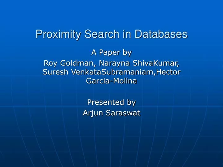
Proximity Search in Databases. A Paper by Roy Goldman, Narayna ShivaKumar, Suresh VenkataSubramaniam,Hector Garcia-Molina Presented by Arjun Saraswat. Flow of the Presentation. Introduction Motivation Problem Statement Model/Design Scoring Function Implementation Strategies

E N D
Proximity Search in Databases A Paper by Roy Goldman, Narayna ShivaKumar, Suresh VenkataSubramaniam,Hector Garcia-Molina Presented by Arjun Saraswat
Flow of the Presentation • Introduction • Motivation • Problem Statement • Model/Design • Scoring Function • Implementation • Strategies • Performance Experiments
Introduction • Basic Idea: Proximity search is used in IR to retrieve documents that have words occurring near each other. • Database is viewed as a collection of objects that are related by distance function. • Objects: can be tuples, records… • In IR traditionally intra-object proximity search is searching within the same document. • The Proximity search in this paper talks about ranking objects based on their distance to other objects.
Motivation • There are situations in which user cannot generate a specific query or its impractical to generate a specific query, or even when a search needs to be based on relevance of different data objects • There is no feature in databases and IR for implementation of proximity search . • Motivation is to develop a general purpose proximity service that can be implemented independent of underlying database.
Problem Statement Basic Statement: To rank objects in one given set (Find) based on their proximity to the objects in the another set (near) What is Find Set? It is a set that is basically of interest for the Proximity search. What is Near Set ? Ranking of Find set objects is done in respect of their distance to Near set objects. Gets more clear with example: “ Find Movie Near Travolta Cage”
Problem Statement Find Movie Looks for all objects of the type movie or the objects that have word movie in there body ,it does not in anyway means that it will search for a movie containing Travolta and Cage Here Movie, Travolta and Cage all are different objects. For the Query “Find Movie Near TravoltaCage” The Top 10 results are: 1.Face off 2.She’s so Lovely 3.Primary colors 4.Con air 5.Mad City 6.Happy Birthday Elizabeth: A Celebration for life 7.Original Sin’s 8.’Night Sins’ 9. That old feeling 10. Dancer Upstairs
Problem Statement As we can clearly see that “Face-off” is going to be the top hit as it has both the stars Travolta and Cage. This can be explained as both actor objects are at a short distance away from the movie Face-off. The movies in second place are here 5 in number, they all have one of the two stars. Rest of the answers have an indirect affiliations means they are at a larger distances.
Model/Design • Figure .1 gives a clear view of the basic components of the Proximity Search architecture • A database stores a set of objects that can be tuples, records, etc. • The application fires Find and Near Queries to get the Find set and the Near set • The Proximity Search Engine takes input as Find and Near objects or sets and Distance Module and gives output as re-ranked Find Set based on there distances, which is obtained from the Distance Module.
Model/Design Distance Module in simplified terms can be understood as providing the Proximity Search Engine with set of triplets like (X, Y, d) where d is the distance between objects with identifiers X and Y. Assumption1: all distances are taken to be greater than or equal to one. Assumption2: Proximity Search Engine makes use of these distances to compute the lengths of shortest paths between objects. Now, As we are more interested in close objects we disregard all objects with distances greater than some constant K and setting an infinity for the rest. will become more clear when we talk about thealgorithm
Model/Design From the perspective of Proximity Search engine the database is viewed as undirected graph with weighted edges. It does not mean that the underlying databases need to be maintained as an undirected graph. As can be seen from the figure given on the right side which shows a normalized relational schema for the Internet Movie Database.
Model/Design In the graph based the representation each tuple is broken down into multiple objects: one for the entity object and additional objects for each attribute value. The distances are assigned between objects are done on the following basis: 1.Small weights are assigned between objects like entity and its attribute values i.e. a close relationship. 2.Larger weights to objects linked through foreign and primary keys. 3.Largest weights are assigned to objects linked by entity tuples in the same relation.
Scoring Function The main idea behind all this is that we want to rank each object f in the Find set based on there proximity to the to the objects in the Near set N. rF : ranking function in the Find set. rN : ranking function in the Near set. range for these functions is [0,1] with 1 representing the highest possible rank. The distance between any two objects f ЄF and n ЄN is the weight of the shortest distance in the underlying database graph, known as d (f, n) .Bond between f and n where f ≠ n : rF(f) rN(n) b (f, n) = d (f, n)t here t is a tuning exponent, it is non-negative real number that controls the impact of distance on bond
Scoring Function The Bond ranges between [0,1], higher the value greater is the bond How to use Bond’s depends upon the application, different approaches can be taken for interpreting bonds to Near objects Some of the approaches are discussed below: 1.Additive : For example in the Query “Find Movie Near TravoltaCage” we intuitively know that movie that has both the actors should be ranked higher so in accordance to our intuition we score each object f based on the sum of its bonds with Near objects score (f) = nЄN Σ b (f, n)
Scoring Function 2.Maximum : In some cases maximum bond may be more important than the total number, in this case score (f) = nЄN max b (f, n) 3.Beliefs : In this we treat bonds as beliefs, that is suppose the graph represents a connection between electronic devices, such that the two devices close together in the graph are close together physically as well. Here rF : indicates the known status of the Find Devices rN: gives that a Near device is faulty b (f ,n) gives us the belief that f is faulty due to n, as the more closer f is to faulty device more likely it is to be faulty score (f) = 1- nЄNΠ (1-b (f, n))
Implementation The implementation of the proximity search architecture was done on top of LORE a database system that was designed at Stanford University for storage and querying graph structured data. It is based on OEM (Object Exchange Model) What is OEM ? • An OEM object contains an OID, textual label, a type and a value. • A value may be atomic or complex. • Atomic OEM any data value that should be considered indivisible by the database • A complex OEM value, on the other hand, is a collection of 0 or more OEM objects
Implementation Complex OEM Object: <Birthday { <Month "January"> <Day 7> <Year 1972> }> Here Birthday is the single complex OEM object with three Atomic OEM objects Month, Day and Year
Implementation Basics of OEM : <Restaurant { <Entree {<Name "Burger"> <NINE: Price 9.00>}> <Entree {<Name "BLT"> <&NINE>}> <Entree {<Name "Reuben"> <Cost &NINE>}> }> Here NINE is SymOid
Strategies Naïve Approach : A simple approach would be to compute the shortest distances between the objects at search time using the Dijkstra's single source shortest path algorithm. For each iteration the algorithm will explore N(v) Vertices adjacent to the some vertex v, so it will Make N(v) random seeks for a disk based graph and as many as |E1| random seeks. This type of approach Requires too many random seeks . E1 : edge list provided by the distance module, it is of the form <u,v,w>
StrategiesAlgorithm for Self joins Algorithm: Distance self-join Input: Edge set El, Maximum required distance: K Output: Lookup table Dist supplies the shortest distance (up to K) between any pair of objects [1] For l = 1 to ┌log2k ┐ [2] Copy El into El’+1 [3] Sort El on first vertex.// To improve performance [4] Scan sorted El: [5] For each <vi, vJ, wk> and <vi, v’J, w’k> where vj != v’j [6] If (wk + w’k ≤ 2l ) and (wk + w’k ≤ K) [7] Add < vj, v’j, wk + w’k > and < v’j, vj, wk + w’k > to El’+1 [8] Sort on El’+1 first vertex, and store in El’+1 [9] Scan sorted El’+1 : [10] Remove tuple <u, v, w>, if there exists another tuple <u, v, w’>, with w > w’. [11] Let Dist be the final El+1. [12] Build index on first vertex in Dist.
Strategies In algorithm for self joins • El: edge-list representation of A2l-1 • El’: edge-list before applying min operator • The algorithm is iterated┌log2k┐and gives the square of the original matrix ┌log2k┐times to give the Ak • The final output that is Dist is the look-up table that contains the distances of all k neighborhood vertices. • The table stores <vi, vJ, wk> for all vertex pairs vi, vJ having wk ≤ K • The main purpose is to query for d(vi, vJ) which can be done efficiently as the Dist table is indexed and access of neighborhood for a tuple like <vi, vJ, wk> ,if its there then distance is wk or distance is greater than K. • The problem with this approach is that it requires a lot of space for the generated edge-list and scanning & sorting operation on it can be expensive.
Strategies • Hub Indexing : It requires far less space for shortest distances then self join algorithm at the cost of access time. • Hubs : Here in the figure p and q are hub vertices that connect to two sub graphs called as hubs Here we calculate for (|A| + |B|) pair wise shortest distances rather than storing all (|A| * |B|).
Strategies Construction of hub indexes : Main Components are a Hub Set H and Table of distances whose shortest path do not cross through H The DIST look-up table that was generated by the Self-Join algorithm. In that one step needs to be changed to make the algorithm in accordance to Hub indexes, that is
Strategies We need to maintain a matrix of pair-wise of hubs in Memory of the form Hubs [hi] [hj] , initializing with distances equal to infinity ,and for each edge <hi, hj, wk> where hi, hj Є H, Hubs [hi] [hj] = wk Floyd Warshall’s algorithm is used to compute shortest distances in hubs.
Strategieshub indexing algorithm • Algorithm: Pair-wise distance querying • Input: Lookup table on disk: Dist, Lookup matrix in memory: Hubs, Maximum required distance: K, Hub set: H • Vertices to compute distance between: u, v (u≠ v) • Return Value: Distance between u and v: d [1] If u, v Є H, return d =Hubs [u ][v]. [2] d = ∞ [3] If u Є H [4] For each <v, vi, wk> in Dist [5] If viЄ H // Path u ~vi~ v [6] d = min (d, wk+ Hubs [vi ] [ u ]) [7] If d > K, return d = ∞, else return d. [8] Steps [4]-[7] are symmetric steps if v Є H, and u !Є H. [9] // Neither u nor v is in H [10] Cache in main-memory (EU) all <u, vi, wk > from Dist [11] For each <v, v’i ,w’k > in Dist [12] If (v’i = u) [13] d = min(d,w’k) //Path u ~ v without crossing hubs [14] For each edge <u, vi, wk > in EU [15] If v’iЄ H and viЄ H //Path u~ vi ~ v’i ~v [16] d = min (d, wk+ w’k +Hubs [v’I] [vi] ) [17] If d > K, return d = ∞, else return d.
Strategies • The algorithms discussed earlier on can be used to get the distances between single pair of objects • Naïve approach for Find/Near Query would be to check for the all pairs of Find and Near objects. To avoid unnecessary seeks clustering over the objects can be done this has to be done engine administrator. • In this Proximity search engine clustering is done on the labels such as Actors, Producers, etc.
Strategies Hub Selection Consider a Graph G(V,E) , and let V1, V2 be disjoint Subsets of V, A set of vertices S ⊆ V separates V1 & V2 If all pairs vertices (v1, v2) v1 Є V1 , v2 Є V2 goes thru some Vertex from S. We say that S is a balanced separator if min(|V1||V2|) ≥ |V|/3 We say that S is a c-separator if V - S = V1 U V2, i.e. S disconnects the graph
Performance Experiments • For the experiments, they have used a Sun SPARC/Ultra II (2x200 MHz) running SunOS 5.6, with 256 MBs of RAM, and 18 GBs of local disk space. • They have done experiments with two sets of datasets IMDB and DBgroup dataset.
Performance Experiments • A generator is used that takes in as input as IMDB’s edge list and scales the database by a scale factor S. • For performance we have user ISAM indexes Performance Issues discussed: Index Performance : • First figure is storage requirements with varying K • Second figure is Index Construction time for varying K • When the number of Hubs is small • For this we have taken the scale Factor to be S =10 and 2.5% vertices as hubs
Performance Experiments • Algorithm Scalability as database grows in size. • First figure is total storage with varying scale . • For this scale factor is taken to be S =10 and 2.5% vertices as hubs. • Second figure number of hubs as percentage of vertices. • For this scale factor is taken to be K=12,S =10 and 2.5% vertices as hubs.
References 1. A Standard Textual Interchange Format for the Object Exchange Model (OEM) by Roy Goldman, Sudarshan Chawathe, Arturo Crespo, Jason McHugh