Download
1 / 19
210 likes | 628 Views
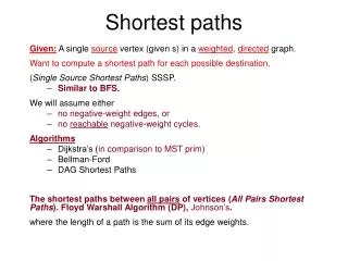
0. A. 4. 8. 2. 8. 2. 3. 7. 1. B. C. D. 3. 9. 5. 8. 2. 5. E. F. Shortest Paths. Outline and Reading. Weighted graphs ( § 7.1) Shortest path problem Shortest path properties Dijkstra’s algorithm ( § 7.1.1) Algorithm Edge relaxation The Bellman-Ford algorithm ( § 7.1.2)

E N D
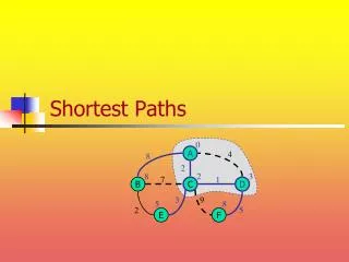
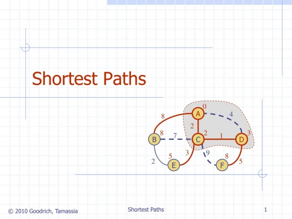
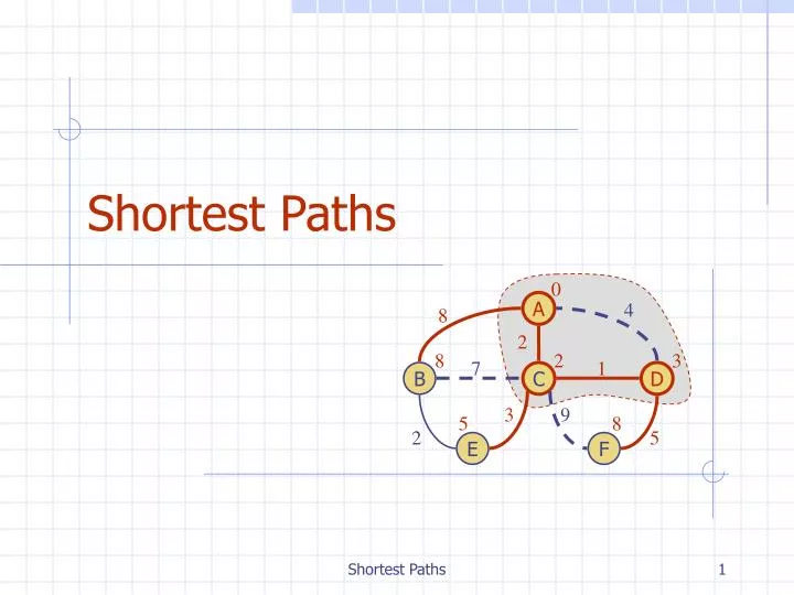
0 A 4 8 2 8 2 3 7 1 B C D 3 9 5 8 2 5 E F Shortest Paths Shortest Paths
Outline and Reading • Weighted graphs (§7.1) • Shortest path problem • Shortest path properties • Dijkstra’s algorithm (§7.1.1) • Algorithm • Edge relaxation • The Bellman-Ford algorithm (§7.1.2) • Shortest paths in dags (§7.1.3) • All-pairs shortest paths (§7.2.1) Shortest Paths
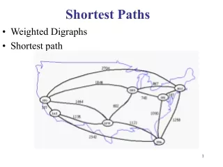
Weighted Graphs • In a weighted graph, each edge has an associated numerical value, called the weight of the edge • Edge weights may represent, distances, costs, etc. • Example: • In a flight route graph, the weight of an edge represents the distance in miles between the endpoint airports 849 PVD 1843 ORD 142 SFO 802 LGA 1205 1743 337 1387 HNL 2555 1099 1233 LAX 1120 DFW MIA Shortest Paths
Shortest Path Problem • Given a weighted graph and two vertices u and v, we want to find a path of minimum total weight between u and v. • Length of a path is the sum of the weights of its edges. • Example: • Shortest path between Providence and Honolulu • Applications • Internet packet routing • Flight reservations • Driving directions 849 PVD 1843 ORD 142 SFO 802 LGA 1205 1743 337 1387 HNL 2555 1099 1233 LAX 1120 DFW MIA Shortest Paths
Shortest Path Properties Property : A subpath of a shortest path is itself a shortest path Single-source shortest paths: Given a weighted graph G and a vertex (s) of G, we are asked to find a shortest path from s to each other vertex in G. All such single-source shortest paths (if they exist) will from a tree. Example: Tree of shortest paths from Providence 849 PVD 1843 ORD 142 SFO 802 LGA 1205 1743 337 1387 HNL 2555 1099 1233 LAX 1120 DFW MIA Shortest Paths
The distance of a vertex v from a vertex s is the length of a shortest path between s and v Dijkstra’s algorithm computes the distances from a given start vertex sto all the other vertices Assumptions: the graph is connected the edges are undirected the edge weights are nonnegative We grow a “cloud” of vertices, beginning with s and eventually covering all the vertices We store with each vertex v a label d(v), which stores the length of the best path that we can find from s to v if we only considerthe subgraph consisting of the cloud and its adjacent vertices At each step We add to the cloud the vertex u outside the cloud with the smallest distance label, d(u) We update the labels of the vertices that are adjacent to uand are outside of the cloud,(edge relaxation) Dijkstra’s Algorithm Shortest Paths
Edge Relaxation • Consider an edge e =(u,z) such that • uis the vertex most recently added to the cloud • z is not in the cloud • The relaxation of edge e updates distance d(z) as follows: d(z)min{d(z),d(u) + weight(e)} d(u) = 50 d(z) = 75 10 e u z s d(u) = 50 d(z) = 60 10 e u z s Shortest Paths
0 A 4 8 2 8 2 3 7 1 B C D 3 9 5 8 2 5 E F Example 0 A 4 8 2 8 2 4 7 1 B C D 3 9 2 5 E F 0 0 A A 4 4 8 8 2 2 8 2 3 7 2 3 7 1 7 1 B C D B C D 3 9 3 9 5 11 5 8 2 5 2 5 E F E F Shortest Paths
Example (cont.) 0 A 4 8 2 7 2 3 7 1 B C D 3 9 5 8 2 5 E F 0 A 4 8 2 7 2 3 7 1 B C D 3 9 5 8 2 5 E F Shortest Paths
Dijkstra’s Algorithm AlgorithmDijkstraShortestDistances(G, v) Input: A simple undirected graph G with nonnegative edge weights and a vertex v. Output: A label D[u] for each vertex u, such that D[u] is the shortest distance from v to u in G for all u G.vertices() ifu= v D[u]0; else D[u]+; Let Q be a priority queue that contains all the vertex of G using D labels as keys. . while Q.isEmpty() u Q.removeMin() for each vertex z adjacent to u such that z is in Q ifD[z]< D[u]+w(u,z)thenD[z]D[u]+w(u,z) Change to D[z] the key of z in Q Return D[u] for every u Shortest Paths
Graph operations Method incidentEdges (to find the adjacent vertices) is called once for each vertex Label operations For each vertex z, We set/get the D[z]O(deg(z)) times Each Set/get of D[z] takes O(1) time Priority queue operations Each vertex is inserted once into and removed once from the priority queue, where each insertion or removal takes O(log n) time The key of a vertex in the priority queue is modified at most deg(w) times, where each key change takes O(log n) time Dijkstra’s algorithm runs in O((n + m) log n) time provided the graph is represented by the adjacency list structure Recall that Sv deg(v)= 2m The running time can also be expressed as O(m log n)since the graph is simple and connected Analysis Shortest Paths
Extension AlgorithmDijkstraShortestPathsTree(G, s) … for all v G.vertices() … P[v]= … while Q.isEmpty() u Q.removeMin() • for each vertex z adjacent to u such that z is in Q • ifD[z]< D[u]+weight(u,z)then • D[z]D[u]+weight(u,z) • Change to D[z] the key of z in Q P[z]=edge(u,z) … • Using the template method pattern, we can extend Dijkstra’s algorithm to return a tree of shortest paths from the start vertex to all other vertices • We store with each vertex z a trace-back label P[z]: • The parent edge in the shortest path tree • In the edge relaxation step, we update P[Z] Shortest Paths
Why Dijkstra’s Algorithm Works • Dijkstra’s algorithm is based on the greedy method. It adds vertices by increasing distance. • Lemma 7.1 In Dijkstra’s algorithm, whenever a vertex u is pulled into the cloud, the label D[u] is equal to the length of the shortest path from v to u. • Suppose Lemma 7.1 is not correct. Let F be the first wrong vertex the algorithm processed. Then D[F] is not equal to the length of shortest path from s to F, when F is pulled into the cloud. • Let D be the previous nodeon the true shortest path. • When D is in the cloud • When D is not in the cloud 0 A 4 8 2 7 2 3 7 1 B C D 3 9 5 8 2 5 E F Shortest Paths
Why It Doesn’t Work for Negative-Weight Edges Dijkstra’s algorithm is based on the greedy method. It adds vertices by increasing distance. • If a node with a negative incident edge were to be added late to the cloud, it could mess up distances for vertices already in the cloud. 0 A 4 8 6 7 5 4 7 1 B C D 0 -8 5 9 2 5 E F C’s true distance is 1, but it is already in the cloud with d(C)=5! Shortest Paths
Bellman-Ford Algorithm AlgorithmBellmanFord(G, s) for all v G.vertices() ifv= s setDistance(v, 0) else setDistance(v, ) for i 1 to n-1 do for each e G.edges() { relax edge e } u G.origin(e) z G.opposite(u,e) r getDistance(u) + weight(e) ifD[u]+weight(e)< d(z) d[z]= D[u]+weight(e) • Works even with negative-weight edges • Must assume directed edges (for otherwise we would have negative-weight cycles) • Iteration i finds all shortest paths that use i edges. • Running time: O(nm). • Can be extended to determine whether the graph contains a negative-weight cycle • How? Shortest Paths
Bellman-Ford Example Nodes are labeled with their d(v) values 0 0 4 4 8 8 -2 -2 -2 4 8 7 1 7 1 3 9 3 9 -2 5 -2 5 0 0 4 4 8 8 -2 -2 7 1 -1 7 1 5 8 -2 4 5 -2 -1 1 3 9 3 9 6 9 4 -2 5 -2 5 1 9 Shortest Paths
Shortest Paths in DAG • If the weighted graph is a DAG, we can solve the single-source shortest paths problem faster. • Compute the topological ordering in O(n+m) • Given the topological ordering, all shortest paths from a vertex can be computed in O(n+m) Shortest Paths
Shortest Paths in DAG Algorithm DAGShortestPath(G,s) Input: a weighted DAG with vertices and m edges. s is a vertex. Output: A label D[u] for each vertex u of G, such that D[u] is the shortest distance from v to u in G. Compute a topological ordering (v1, v2,,,vn) for G D[s]o For each vertex u≠s D[s]+ For i1 to n-1 do {relax each outgoing eadge from vi} for each edge (vi, u) outgoing from vi do if D[vi]+w((vi, u))<D[u] then D[u] D[vi]+w((vi, u)) Output the distance labels D as the distances from s. Shortest Paths
All-Pairs Shortest Paths AlgorithmAllPair(G) {assumes vertices 1,…,n} for all vertex pairs (i,j) ifi= j D0[i,i] 0 else if (i,j) is an edge in G D0[i,j] weight of edge (i,j) else D0[i,j] + for k 1 to n do for i 1 to n do for j 1 to n do Dk[i,j] min{Dk-1[i,j], Dk-1[i,k]+Dk-1[k,j]} return Dn • Find the shortest distance between every pair of vertices in a weighted directed graph G. • We can make n calls to Dijkstra’s algorithm (if no negative edges), which takes O(nmlog n) time. • Likewise, n calls to Bellman-Ford would take O(n2m) time. • We can achieve O(n3) time using dynamic programming (similar to the Floyd-Warshall algorithm). Uses only vertices numbered 1,…,k (compute weight of this edge) i j Uses only vertices numbered 1,…,k-1 Uses only vertices numbered 1,…,k-1 k Shortest Paths