Download

1 / 36
360 likes | 538 Views
Image-Guided Weathering: A New Approach Applied to Flow Phenomena. C. Bosch 1 , P. Y. Laffont, H. Rushmeier, J. Dorsey, G. Drettakis Yale University – REVES/INRIA Sophia Antipolis 1 Currently at ViRVIG, University of Girona. Aging and Weathering. Essential for modeling urban environments

E N D
Image-Guided Weathering:A New Approach Applied to Flow Phenomena C. Bosch1, P. Y. Laffont, H. Rushmeier, J. Dorsey, G. Drettakis Yale University – REVES/INRIA Sophia Antipolis 1 Currently at ViRVIG, University of Girona
Aging and Weathering • Essential for modeling urban environments • Governed by physical, chemical and biological processes
Flow effects • Particularly complex • Flow over the scene (global effect) • Material properties (local effect)
Aging and Weathering in CG • Physically-based simulation • Difficult to get the desired effect • Texture synthesis • Restricted by input information • Global effects particularly hard
Motivation • Physically-based simulation • More flexible, allows global effects • Two main difficulties • Choosing appropriate parameters to achieve a given effect • Obtaining realistic visual detail
Image-Guided Weathering • Use images to guide simulation • Flow stains as a representative case Exemplar New simulation
Overview (I) • Extract data from exemplars • Color information • Simulation parameters • High frequency details Si= 1.301 rt = 0.252 kS = 0.0201 at = 0.404 kD = 0.0807 T = 803 ka,t = 0.021 Exemplar Data
Overview (II) • Simulate new effects on scenes Si= 1.301 rt = 0.252 kS = 0.0201 at = 0.404 kD = 0.0807 T = 803 ka,t = 0.021 Data
Related Work • Simulation • Phenomenon-specific [Merillou08] • Flow stains [Dorsey96; Chen05; Endo10] • Capture-and-transfer (synthesis) • Single image [Wang06; Xue08] • Acquisition systems [Gu06; Mertens06; Sun07; Lu07] • Inverse procedural textures [Bourque04; Lefebvre00]
Flow model • Particle-based simulation [Dorsey96] • Absorption, solubility and deposition • Stain concentration maps • Parameters • Particles: mass (m), Si • Stain material: kS, kD • Target materials: a, ka, roughness (r) • Simulation: time (t), particle rate (N)
Extracting Stains • Based on Appearance Manifolds [Wang06] Appearance Manifold Exemplar Degree Map
Simulation Error Parameter Fitting Proxy geometry • Degree map = Stain concentration map Input stain Degree map source target Initial parameters Si= 1 kS = 0.04 kD= 0.04 rt= 0.2 at= 0.3 ka,t = 0.05 T = 300 image plane Si= 1.3 kS = 0.02 kD= 0.08 rt= 0.25 at= 0.4 ka,t = 0.02 T = 803 Error < threshold or max. iterations (Levenberg-Marquardt) [Lourakis04] Stop New parameters
Improving Fitting • Stain distribution along the source • Accumulate degree from bottom to top
Improving Fitting (II) • Flow deflection along the target • Compute local degree distribution (~vector field)
Simulation Error Parameter Fitting (II) Proxy geometry Stain distribution Input stain Degree map source target Initial parameters Vector field Si= 1 kS = 0.04 kD= 0.04 rt= 0.2 at= 0.3 ka,t = 0.05 T = 300 image plane Si= 1.3 kS = 0.02 kD= 0.08 rt= 0.25 at= 0.4 ka,t = 0.02 T = 803 Error < threshold or max. iterations (Levenberg-Marquardt) [Lourakis04] Stop New parameters
Fitting Results (w/o vector field) Using source distribution Exemplar Degree Map Simulation
Fitting Results (w/o vector field) Exemplar Degree Map Simulation
Fitting Results (w/ vector field) Exemplar w/o vfield Degree Map Simulation
Fitting Results (w/ vector field) Exemplar Degree Map Simulation
Fitting Results (w/ vector field) Exemplar Degree Map Simulation
Fitting Results (Complex Targets) Exemplar Degree Map Simulation
Stain Detail • Simulation lacks spatial variations (high-frequency detail) Degree Map Simulation Exemplar
Detail Maps • Extract detail by image difference • Use guided texture synthesis [Lefebvre05] • Detail maps will modify stain adhesion Detail Map Degree Map Simulation Difference
Simulating New Stains • Link data to stain sources and targets • Parameters, detail maps, color • Use 1D texture synthesis for distributions • Run flow simulation • Flow deflected by target geometry (+ disp. map)
Color Transfer target background • Transfer stain color from input image • Background mixed with stain everywhere • Non-linear relationship between color and degree • Use per-pixel warping background color fully stained
Performance • Preprocessing • Degree map: 1-3 minutes • Fitting: 30-60 minutes (500 iter., ~256x512) • Detail synthesis: 1-2 minutes (1024x1024) • Final simulation • Stain simulation: 2-5 minutes/stain • Color warping: 5-8 seconds/stain (1024x1024)
Limitations • Good extraction from background • Fitting: Not true physical estimations • Detail maps: Depend on appropriate fit • Computation time
Conclusions • New approach to acquire simulation data from photographs • Solves parameter estimation from images • Combines simulation with data-driven methods • Appearance manifold, texture synthesis, … • Fills the gap between data-driven and simulation Easy to use Natural variations (including global effects)
Future work • Extend to other weathering phenomena • Deal with large scale scenes • Fast simulation, global effects, …
Acknowledgements • Visiting grant U.Girona • ANR project (ANR-06-MDCA-004-01) • ERCIM “Alain Bensoussan” Fellowship • Autodesk (Maya/MentalRay) • Coding help: Li-Ying, Su Xue • Scene treatment: S. Close and F. Andrade-Cabral