Download
1 / 43
430 likes | 588 Views
Rounding-based Moves for Metric Labeling. M. Pawan Kumar École Centrale Paris INRIA Saclay , Île-de-France. Metric Labeling. Variables V = { V 1 , V 2 , …, V n }. Metric Labeling. Variables V = { V 1 , V 2 , …, V n }. Metric Labeling. w ab d (f(a),f(b)). θ b (f(b)). w ab ≥ 0.

E N D
Rounding-based Movesfor Metric Labeling M. Pawan Kumar ÉcoleCentrale Paris INRIA Saclay, Île-de-France
Metric Labeling Variables V= { V1, V2, …, Vn}
Metric Labeling Variables V= { V1, V2, …, Vn}
Metric Labeling wabd(f(a),f(b)) θb(f(b)) wab ≥ 0 θa(f(a)) d is metric Va Vb minf E(f) + Σ(a,b)wabd(f(a),f(b)) = Σaθa(f(a)) Labels L= { l1, l2, …, lh} Variables V= { V1, V2, …, Vn} Labeling f: { 1, 2, …, n} {1, 2, …, h}
Metric Labeling Va Vb minf E(f) + Σ(a,b)wabd(f(a),f(b)) = Σaθa(f(a)) NP hard Low-level vision applications
Outline • Approximate Algorithms • Comparison • Rounding-based Moves • Conclusion
Boykov, Veksler and Zabih Efficiency Move-Making Algorithms Kleinberg and Tardos Accuracy Convex Relaxations
Kolmogorov and Zabih Efficiency Move-Making Algorithms Chekuri, Khanna, Naor and Zosin Accuracy Convex Relaxations
Outline • Approximate Algorithms • Move-Making Algorithms • Linear Programming Relaxation • Comparison • Rounding-based Moves • Conclusion
Move-Making Algorithms Space of All Labelings f
Expansion Algorithm Variables take label lα or retain current label Boykov, Veksler and Zabih, 2001 Slide courtesy PushmeetKohli
Expansion Algorithm Variables take label lα or retain current label Tree Ground House Status: Initialize with Tree Expand Ground Expand House Expand Sky Sky Boykov, Veksler and Zabih, 2001 Slide courtesy PushmeetKohli
Multiplicative Bounds f*: Optimal Labeling f: Estimated Labeling Σaθa(f(a)) + Σ(a,b)wabd(f(a),f(b)) ≥ Σaθa(f*(a)) + Σ(a,b)wabd(f*(a),f*(b))
Multiplicative Bounds f*: Optimal Labeling f: Estimated Labeling Σaθa(f(a)) + Σ(a,b)wabd(f(a),f(b)) ≤ B Σaθa(f*(a)) + Σ(a,b)wabd(f*(a),f*(b))
Outline • Approximate Algorithms • Move-Making Algorithms • Linear Programming Relaxation • Comparison • Rounding-based Moves • Conclusion
Integer Linear Program Minimize a linear function over a set of feasible solutions Indicator xa(i) {0,1} for each variable Va and label li Indicator xab(i,k) {0,1} for each neighbor (Va,Vb) and labels li, lk Number of facets grows exponentially in problem size
Linear Programming Relaxation Indicator xa(i) {0,1} for each variable Va and label li Indicator xab(i,k) {0,1} for each neighbor (Va,Vb) and labels li, lk Schlesinger, 1976; Chekuri et al., 2001; Wainwright et al., 2003
Linear Programming Relaxation Indicator xa(i) [0,1] for each variable Va and label li Indicator xab(i,k) [0,1] for each neighbor (Va,Vb) and labels li, lk Schlesinger, 1976; Chekuri et al., 2001; Wainwright et al., 2003
Approximation Factor x*: LP Optimal Solution x: Estimated Integral Solution ΣaΣiθa(i)xa(i) + Σ(a,b)Σ(i,k) wabd(i,k)xab(i,k) ≥ ΣaΣiθa(i)x*a(i) + Σ(a,b)Σ(i,k) wabd(i,k)x*ab(i,k)
Approximation Factor x*: LP Optimal Solution x: Estimated Integral Solution ΣaΣiθa(i)xa(i) + Σ(a,b)Σ(i,k) wabd(i,k)xab(i,k) ≤ F ΣaΣiθa(i)x*a(i) + Σ(a,b)Σ(i,k) wabd(i,k)x*ab(i,k)
Outline • Approximate Algorithms • Comparison • Rounding-based Moves • Conclusion
Theoretical Guarantees M = ratio of maximum and minimum non-zero distance
Outline • Approximate Algorithms • Comparison • Rounding-based Moves • Conclusion
Interval Rounding Treat xa(i) [0,1] as probability that f(a) = i Cumulative probability ya(i) = Σj≤ixa(j) ya(2) ya(i) ya(k) 0 ya(1) ya(h) = 1 Choose an interval of length h’
Interval Rounding Treat xa(i) [0,1] as probability that f(a) = i Cumulative probability ya(i) = Σj≤ixa(j) r 0 ya(k)-ya(i) REPEAT Choose an interval of length h’ Generate a random number r (0,1] Assign the label next to r if it is within the interval
Example 0.25 0.5 0.75 1.0 ya(2) ya(3) 0 ya(1) ya(4) 0.7 0.8 0.9 1.0 yb(1) yb(3) 0 yb(4) yb(2) 0.2 0.3 0.1 1.0 0 yc(3) yc(2) yc(4) yc(1)
Example 0.25 0.5 r ya(2) 0 ya(1) 0.7 0.8 r yb(1) 0 yb(2) 0.2 0.1 r 0 yc(2) yc(1)
Example 0.25 0.5 0.75 1.0 ya(2) ya(3) 0 ya(1) ya(4) 0.7 0.8 0.9 1.0 yb(1) yb(3) 0 yb(4) yb(2) 0.2 0.3 0.1 1.0 0 yc(3) yc(2) yc(4) yc(1)
Example 0.2 0.3 0.1 1.0 0 yc(3) yc(2) yc(4) yc(1)
Example 0.1 0.2 r yc(3) yc(2) 0 -yc(1) -yc(1)
Example 0.25 0.5 0.75 1.0 ya(2) ya(3) 0 ya(1) ya(4) 0.7 0.8 0.9 1.0 yb(1) yb(3) 0 yb(4) yb(2) 0.2 0.3 0.1 1.0 0 yc(3) yc(2) yc(4) yc(1)
Key Observation If d is submodular d(i,k) + d(i+1,k+1) ≤ d(i,k+1) + d(i+1,k), for all i, k energy can be minimized via minimum cut Schlesinger and Flach, 2003
Interval Move Choose an interval of length h’ Va Vb θab(i,k) = wabd(i,k)
Interval Move Choose an interval of length h’ Add the current labels Va Vb θab(i,k) = wabd(i,k)
Interval Move Choose an interval of length h’ Add the current labels d’(i,k) ≥ d(i,k) d’ is submodular Solve to update labels Va Vb Repeat until convergence θab(i,k) = wabd’(i,k)
Interval Move Each problem can be solved using minimum cut Same multiplicative bound as interval rounding Multiplicative bound is tight
Outline • Approximate Algorithms • Comparison • Rounding-based Moves • Conclusion
Theoretical Guarantees M = ratio of maximum and minimum non-zero distance
Boykov, Veksler and Zabih Length of interval = 1 Move-Making Algorithms Kleinberg and Tardos Length of interval = 1 Convex Relaxations
Boykov, Veksler and Zabih Length of interval = 1 Move-Making Algorithms Chekuri, Khanna, Naor and Zosin Optimal interval length Convex Relaxations
Theoretical Guarantees M = ratio of maximum and minimum non-zero distance
Questions? http://cvn.ecp.fr/personnel/pawan pawan.kumar@ecp.fr