Download
1 / 51
520 likes | 766 Views
Hardware and Petri nets. Partial order methods for analysis and verification of asynchronous circuits. Outline. Representing Petri net semantics with occurrence nets (unfoldings) Unfolding (finite) prefix construction Analysis of asynchronous circuits Problems with efficient unfolding.

E N D
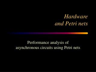
Hardwareand Petri nets Partial order methods foranalysis and verification of asynchronous circuits
Outline • Representing Petri net semantics with occurrence nets (unfoldings) • Unfolding (finite) prefix construction • Analysis of asynchronous circuits • Problems with efficient unfolding
Approaches to PN analysis • Reachable state space: • Direct or symbolic representation • Full or reduced state space (e.g. stubborn set method) in both cases knowledge of Petri net structural relations (e.g. conflicts) helps efficiency • Unfolding the Petri net graph into an acyclic branching graph (occurrence net), with partial ordering between events and conditions and: • Considering a finite prefix of the unfolding which covers all reachable states and contains enough information for properties to be verified
p1 Petri net t1 t2 p2 p4 p5 p3 p1 t4 t5 t3 t6 t1 t2 p6 p6 p7 p7 t7 t7 p4 p5 p2 p3 p1 p1 t6 t4 t5 t3 t1 t2 t1 t2 p2 p2 p4 p4 p5 p3 p5 p3 t4 t5 p7 t4 t5 p6 t3 t3 t6 t6 p6 p6 p7 p7 p7 p7 t7 … … … … Occurrence nets Min-place Occurrence net
t3 t5 (1) p6 p1 (2) t2 t1 infinite set t p7 p6 p1 p2 t7 t7 t (4) (3) Occurrence nets • The occurrence net of a PN N is a labelled (with names of the places and transitions of N) net (possibly infinite!) which is: • Acyclic • Contains no backward conflicts (1) • No transition is in self-conflict (2) • No twin transitions (3) • Finitely preceded (4) NO! NO! NO! NO!
Relations in occurrence nets p1 conflict t1 t2 p2 p4 p5 p3 precedence t4 t5 t3 t6 p6 p6 p7 p7 concurrency t7 t7 p1 p1 t1 t2 t1 t2 p2 p2 p4 p4 p5 p3 p5 p3 t4 t5 t4 t5 t3 t3 t6 t6 p6 p6 p7 p7 p7 p7
Unfolding of a PN • The unfolding of Petri net N is a maximal labelled occurrence net (up to isomorphism) that preserves: • one-to-one correspondence (bijection) between the predecessors and successors of transitions with those in the original net • bijection between min places and the initial marking elements (which is multi-set) p’ p’’ p p7 p6 p7’ p6’ t7 t7’ unfolding N’ net N net N unfolding N’
t1 t2 t2 p2 p4 p4 p5 p5 p3 t5 t6 t3 t4 t3 p6 p7 p6 p7 t7 t7 p1 p1 Unfolding construction p1 p1 t1 p2 p3 t6 t4 t5 p7 p6 t7 and so on …
p1 t1 t2 p2 p4 p5 p3 t4 t5 t3 t6 p6 p6 p7 p7 t7 t7 p1 p1 t1 t2 t1 t2 p2 p2 p4 p4 p5 p3 p5 p3 t4 t5 p7 t4 t5 p6 t3 t3 t6 t6 p6 p6 p7 p7 p7 p7 t7 … … … … Unfolding construction Unfolding Petri net p1 t1 t2 p4 p5 p2 p3 t6 t4 t5 t3
t1 t2 t2 p2 p4 p4 p5 p5 p3 t5 t6 t3 t4 t3 p6 p7 p6 p7 t7 t7 p1 p1 Petri net and its unfolding p1 marking cut p1 t1 p2 p3 t6 t4 t5 p7 p6 t7
t1 t2 t2 p2 p4 p4 p5 p5 p3 t5 t6 t3 t4 t3 p6 p7 p6 p7 t7 t7 p1 p1 Petri net and its unfolding p1 marking cut p1 t1 p2 p3 t6 t4 t5 p7 p6 t7
t1 t2 t2 p2 p4 p4 p5 p5 p3 t5 t6 t3 t4 t3 p6 p7 p6 p7 t7 t7 p1 p1 Petri net and its unfolding p1 marking cut p1 t1 p2 p3 t6 t4 t5 p7 p6 t7
t1 t2 t2 p2 p4 p4 p5 p5 p3 t5 t6 t4 p6 p7 p7 t7 p1 Petri net and its unfolding p1 p1 t1 p2 p3 t3 t6 t4 t5 t3 p6 p7 p6 t7 t7 p1 PN transition and its instance in unfolding
t2 t2 p4 p4 p5 p5 p3 t5 t6 p6 p7 t7 p1 Petri net and its unfolding p1 Prehistory (local configuration) of the transition instance p1 t1 t1 p2 p2 p3 t4 t3 t6 t4 t5 t3 p7 p6 p7 p6 t7 t7 p1 Final cut of prehistory and its marking (final state)
t2 t2 p4 p4 p5 p5 p3 t5 t6 p6 p7 t7 p1 Petri net and its unfolding p1 Prehistory (local configuration of the transition instance) p1 t1 t1 p2 p2 p3 t4 t3 t6 t4 t5 t3 p7 p6 p7 p6 t7 t7 p1 Final cut of prehistory and its marking (final state)
Truncation of unfolding • At some point of unfolding the process begins to repeat parts of the net that have already been instantiated • In many cases this also repeats the markings in the form of cuts • The process can be stopped in every such situation • Transitions which generate repeated cuts are called cut-off points or simply cut-offs • The unfolding truncated by cut-off is calledprefix
t1 t2 t2 p2 p4 p4 p5 p5 p3 t5 t6 t3 t3 p6 p7 p6 Cutoff transitions p1 p1 t1 p2 p3 t4 t6 t4 t5 p7 p7 p6 t7 t7 Cut-offs t7 p1 p1
t2 t2 p4 p4 p5 p5 p3 t5 t6 t3 p6 p7 Cutoff transitions p1 p1 pre-history of t7’ t1 t1 p2 p2 p3 t4 t3 t6 t4 t5 p7 p6 p7 p6 t7 t7 Cut-offs t7 p1 p1
Prefix Construction Algorithm ProcBuild prefix (N =<P,T,F,M0>) Initialise N’ with instances of places in M0 Initialise Queue with instances of t enabled at M0 while Queue is not empty do Pull t’ from Queue ift’ is not cutoff then do Add t’ and succ(t’) to N’ for each t in T do Find unused set of mutually concurrent instances of pred(t) ifsuch set existsthen do Add t’ to Queue in order of its prehistory size end do end do end do return N’ end proc
Cut-off definition • A newly built transition instance t1’in the unfolding is a cut-off point if there exists another instance t2’ (of possibly another transition) whose: • Final cut maps to the same marking is the final cut of t1’, and • The size of prehistory (local configuration) of t2’is strictly greater than that of t1’ [McMillan, 1992] • Initial marking and its min-cut are associated with an imaginary “bottom” instance (so we can cut-off on t7 in our example)
t2 t2 p4 p4 p5 p5 p3 t5 t6 t3 t4 t3 p6 p7 p6 p7 Finite prefix p1 p1 t1 t1 p2 p2 p3 t6 t4 t5 p7 p6 t7 t7 t7 For a bounded PN the finite prefix of its unfolding contains all reachable markings [K. McMillan]
Complexity issues • The prefix covers all reachable markings of the original net but the process of prefix construction does not visit all these markings • Only those markings (sometimes called Basic Markings) are visited that are associated with the final cuts of the local configurations of the transition instances • These markings are analogous to primes in an algebraic lattice • The (time) complexity of the algorithm is therefore proportional to the size of the unfolding prefix • For highly concurrent nets this gives a significant gain in efficiency compared to methods based on the reachability graph
Size of Prefix The size of the prefix for this net is O(n) – same as that of the original net while the size of the reachability graph is O(2n) … a1 a2 an • This is however not always true and the size depends on: • the structure and class of the net, and • initial marking b
a1 a2 b2 b1 Size of Prefix p1 p1 a2 a1 p2 p2 p2 b2 b1 b1 b2 p3 p3 p3 p3 p3 c2 c1 c2 c2 c1 c1 c1 c1 c2 c2 p4 p4 cut-off points
a1 a2 Size of Prefix p1 p1 a2 a1 p2 p2 p2 b2 b1 b2 b1 b1 b2 Redundant part p3 p3 p3 p3 p3 c2 c1 c2 c2 c1 c1 c1 c1 c2 c2 p4 p4
1 2 a 3 b 4 c Size of Prefix 1 2 2 a Non-1-safe net a 3 3 b b Cut-offs 4 4 c c 2 2 1 1 However this part is redundant
Cut-off Criteria • McMillan’s cutoff criterion, based on the size of pre-history, can be too strong • A weaker criterion, based only on the matching of the final cuts, was proposed by Esparza, Vogler, and Römer • It uses a total (lexicographical) order on the transition set (when putting them into Queue) • It can be only applied to 1-safe nets because for non-1-safe nets such a total order cannot be established (main reason auto-concurrency of instances of the same transition!) • Unfolding k-safe nets can produce a lot of redundancy
Property analysis • A model-checker to verify a CTL formula (defined on place literals) has been built (Esparza) within the PEP tool (Hildesheim/Oldenburg) • Various standard properties, such as k-boundedness, 1-safeness, persistency, liveness, deadlock freedom have special algorithms, e.g.: • Check for 1-safeness is a special case of auto-concurrency (whether a pair of place instances exist that are mutually concurrent – can be done in polynomial time) • Similar is a check for persistency of some transition (analysis of whether it is in immediate conflict with another transition) • Check for deadlock is exponential (McMillan) – involves enumeration of configurations (non-basic markings), however efficient linear-algebraic techniques have recently been found by Khomenko and Koutny (CONCUR’2000)
STG Unfolding • Unfolding an interpreted Petri net, such as a Signal Transition Graph, requires keeping track of the interpretation – each transition is a change of state of a signal, hence each marking is associated with a binary state • The prefix of an STG must not only “cover” the STG in the Petri net (reachable markings) sense but must also be complete for analysing the implementability of the STG, namely: consistency, output-persistency and Complete State Coding
p1 a+ b+ p2 p3 c+ c+ p4 d+ p5 d- STG Unfolding STG Binary-coded STG Reach. Graph (State Graph) Uninterpreted PN Reachability Graph STG unfold. prefix p1 abcd p1 p1(0000) a+ b+ a+ b+ p3(0100) p2(1000) p2 p3 p2 p3 c+ c+ p4(0110) p4(1010) p4 c+ c+ d+ d+ p4 p4 p5(0111) p5(1011) p5 d+ d+ p5 p5 d- d-
p1 a+ b+ p2 p3 c+ c+ p4 d+ p5 d- STG Unfolding STG Binary-coded STG Reach. Graph (State Graph) Uninterpreted PN Reachability Graph STG unfold. prefix p1 abcd p1 p1(0000) a+ b+ a+ b+ p3(0100) p2(1000) p2 p3 p2 p3 c+ c+ p4(0110) p4(1010) p4 c+ c+ d+ d+ p4 p5(0111) p5(1011) p5 d+ Not like that! p5 d-
p1p6 b+ a+ b- p3p6 p2p6 Consistency and Signal Deadlock STG PN Reach. Graph STG State Graph p1 ab p1p6(00) b+ b+ a+ a+ b- p3p6(01) p2p6(10) p2 p3 a- a- b- p1p4(00) p1p4 b+ a+ b+ a- b- a+ b- b+ b+ p1p5(01) p2p4(10) p3p4 p3p4(01) p2p4 p1p5 p6 p4 b+ b+ b+ b+ b- Signal deadlock wrt b+ (coding consistency violation) p2p5(11) p2p5 p3p5 b+ b- b- b- b- p5
STG p1 b+ a+ p2 p3 a- b- p6 p4 b+ b- p5 Signal Deadlock and Autoconcurrency p6 p1 STG State Graph STG Prefix ab p1p6(00) b+ a+ b+ a+ b- p3p6(01) p3 p2p6(10) p2 a- b- a- b- p1p4(00) b+ p1 a+ b+ p4 p1p5(01) p2p4(10) p3p4(01) b+ b+ p2 b+ a+ Signal deadlock wrt b+ (coding consistency violation) p2p5(11) p5 b- b- p2 b- Autoconcurrency wrt b+
Verifying STG implementability • Consistency – by detecting signal deadlock via autoconcurrency between transitions labelled with the same signal (a* || a*, where a* is a+ or a-) • Output persistency – by detecting conflict relation between output signal transition a* and another signal transition b* • Complete State Coding is less trivial – requires special theory of binary covers on unfolding segments (Kondratyev et.al.)
Experimental results (from Semenov) Example with inconsistent STG: PUNT quickly detects a signal deadlock “on the fly” while Versify builds the state space and then detects inconsistent state coding
Analysis of Circuit Petri Nets Event-driven elements Petri net equivalents C Muller C-element Toggle
Analysis of Circuit Petri Nets • Petri net models built for event-based and level-based elements, together with the models of the environment can be analysed using the STG unfolding prefix • The possibility of hazards is verified by checking either 1-safeness (for event-based) or persistency (for level-based) violations
Circuit Petri Nets Level-driven elements Petri net equivalents Self-loops in ordinary P/T nets y(=0) x=0 x(=1) y=1 y=0 x=1 NOT gate x=0 x(=1) z(=0) z=1 y=0 y(=1) b NAND gate x=1 z=0 y=1
Circuit Petri nets The meaning of these numerous self-loop arcs is however different from self-loops (which take a token and put it back) These should be test or read arcs (without consuming a token) From the viewpoint of analysis we can disregard this semantical discrepancy (it does not affect reachability graph properties!) and use ordinary PN unfolding prefix for analysis, BUT …
Unfolding Nets with Read Arcs PN with self-loops Unfolding with self-loops Unfolding with read arcs Combinatorial explosion due to splitting the self-loops
Unfolding k-safe nets • How to cope with k-safe (k>1) nets and their redundancy • Such nets are extremely useful in modelling various hardware components with: • Buffers of finite capacity • Counters of finite modulo count • McMillan’s cutoff condition is too strong (already much redundancy) • EVR’s condition is too weak – cannot be applied to k-safe nets Proposed solution: introduce total order on tokens, e.g. by applying FIFO discipline of their arrival-departure (work with F.Alamsyah et al.)
Unfolding k-safe Nets Example: producer-consumer
Unfolding k-safe Nets Consider the case: n=1 consumer k=2-place buffer • Three techniques have been studied (by F. Alamsyah): • Direct prefix using McMillan’s cutoff criterion • Unfolding the explicitly refined (with FIFO buffers) 1-safe net (using EVR cutoff criterion) • Unfolding the original, unrefined net with FIFO semantics
Unfolding k-safe Nets Approach (2) for refining FIFO places into 1-safe subnets
Unfolding k-safe Nets (1) Direct unfolding prefix (using McMillan’s cutoff)
Unfolding k-safe Nets (2) Unfolding the explicitly refined (with FIFO buffers) 1-safe net (using EVR’s cutoff)
Unfolding k-safe Nets (2) Unfolding the original, unrefined net with FIFO semantics
Buffer k-bounded net with Mcmillan's unfolding safe nets using ERV's algorithm size Original Unfolding (t/p) time(s) Original Unfolding (t/p) time(s) 2 6/8 184/317 0.05 8/14 29/68 0.03 3 6/8 1098/1896 0.84 10/18 46/105 0.10 4 6/8 6944/11911 21.46 12/22 67/150 0.28 5 6/8 - - 14/26 92/203 0.74 6 6/8 - - 16/30 121/264 1.84 7 6/8 - - 18/34 154/333 4.25 8 6/8 - - 20/38 191/410 8.74 Unfolding k-safe Nets
Buffer safe nets using ERV's algorithm FIFO-unfolding with McMillan's size Original Unfolding (t/p) time(s) Original Unfolding (t/p) time(s) 2 8/14 29/68 0.03 6/8 41/69 0.010 3 10/18 46/105 0.10 6/8 41/68 0.010 4 12/22 67/150 0.28 6/8 51/84 0.020 5 14/26 92/203 0.74 6/8 61/100 0.020 6 16/30 121/264 1.84 6/8 71/116 0.040 7 18/34 154/333 4.25 6/8 81/132 0.050 8 20/38 191/410 8.74 6/8 91/148 0.060 Unfolding k-safe Nets