Download
1 / 65
670 likes | 879 Views
SC968 Panel data methods for sociologists Lecture 1, part 1. A review of concepts for regression modelling Or things you should know already. Overview. Models OLS, logit and probit Mathematically and practically Interpretation of results, measures of fit and regression diagnostics

E N D
SC968Panel data methods for sociologistsLecture 1, part 1 A review of concepts for regression modelling Or things you should know already
Overview • Models • OLS, logit and probit • Mathematically and practically • Interpretation of results, measures of fit and regression diagnostics • Model specification • Post-estimation commands • STATA competence
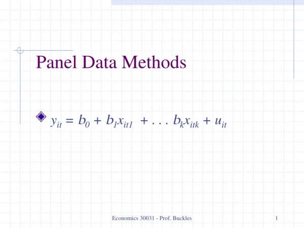
Ordinary Least Squares (OLS) Value of dependent variable for individual i (LHS variable) Residual (disturbance, error term) Intercept (constant) Total no. of explanatory variables (RHS variables or regressors) is K Coefficient on variable 1 Value of explanatory variable 1 for person i Examples yi= mental health x1 = sex x2 = age x3 = marital status x4 = employment status x5 = physical health yi = hourly pay x1 = sex x2 = age x3 = education x4 = job tenure x5 = industry x6 = region
OLS In vector form In matrix form Vector of explanatory variables Vector of coefficients Note: you will often see x’β written as xβ
OLS • Also called “linear regression” • Assumes dependent variable is a linear combination of dependent variables, plus disturbance • “Least squares”: β’s estimated so as to minimise the sum of the ε’s.
Basic Assumptions • Residuals have zero mean………………………………. • Follows that ε’s and X’s are uncorrelated………………. • violated if a regressor is endogenous • Eg, number of children in female labour supply models • Cure by (eg) Instrumental Variables • Homoscedasticity: all ε’s have same variance ………… • Classic example: food consumption and income • Cure by using weighted least squares • Nonautocorrelation: ε’s uncorrelated with each other … • Data sets where the same individual appears multiple times • Adjust standard errors: ‘cluster’ option in STATA • Distubances are iid (normally distributed, zero mean, constant variance)
When is OLS appropriate? • When you have a continuous dependent variable • Eg, you would use it to estimate regressions for height, but not for whether a person has a university degree. • When the assumptions are not obviously violated • As a first step in research to get ball-park estimates • We will use them a lot for this purpose • Worked examples • Coefficients, P-values, t-statistics • Measures of fit (R-squared, adjusted R-squared) • Thinking about specification • Post-estimation commands • Regression diagnostics. • A note on the data • All examples (in lectures and practicals) drawn from a 20% sample of the British Household Panel Survey (BHPS) – more about the data later!
First worked example For illustrative purposes only. Not an example of good practice. Monthly labour income, for people whose labour income is >= £1 MS = SS/df Tests whether all coeffs except constant are jointly zero Analysis of variance (ANOVA) table R-squared = Model SS / Total SS Root MSE = sqrt(MSR) T-stat = coefficient / standard error Coefficients + or – 1.96 standard errors
What do the results tell us? • All coefficients except month of interview are significant • 29% of variation explained • Being female reduces income by nearly £600 per month • Income goes up with age and then down • 16458 observations…..oops, this is from panel data, so there are repeated observations on individuals.
Add ,cluster(pid) as an option • Coefficients, R-squared etc are unchanged from previous specification • But standard errors are adjusted: standard errors larger, t-statistics are lower
Let’s get rid of the “month” variable Think about the female coefficient a bit more. Could it be to do with women working shorter hours?
Control for weekly hours of work • Is the coefficient on hours of work reasonable? • £5.65 for every additional hour worked – certainly in the right ball park.
Looking at 2 specifications together • R-squared jumps from 29% to 46% • Coefficient on female goes from -595 to -315 • Almost half the effect of gender is explained by women’s shorter hours of work • Age, partner and education coefficients are also reduced in magnitude, for similar reasons • Number of observations reduces from 16460 to 13998 – missing data on hours
Interesting post-estimation activities What age does income peak? Income = Y + β1*age + β2*age2 d(Income)/d(age) = β1+ 2β2*age Derivative = zero when age = - β1/2β2 = -79.552/(-0.873*2) = 45.5 Is the effect of university qualifications statistically different from the effect of secondary education?
Men who are part of a couple earn much more than men who are not – women less so. • Other coefficients also differ between men and women, but with current specification, we can’t test whether differences are significant.
Logit and Probit • Developed for discrete (categorical) dependent variables • Eg, psychological morbidity, whether one has a job…. Think of other examples. • Outcome variable is always 0 or 1. Estimate: • OLS (linear probability model) would set F(X,β) = X’β + ε • Inappropriate because: • Heteroscedasticity: the outcome variable is always 0 or 1, so ε only takes the value -x’β or 1-x’β • More seriously, one cannot constrain estimated probabilities to lie between 0 and 1.
Logit and Probit • Solution: We need a link function that will transform our dichotomous Y into a continuous form Y’ • Looking for a function which lies between 0 and 1: • Cumulative normal distribution: Probit model • Z scores assuming the cumulative normal distribution Φ • Logistic distribution: Logit (logistic) model • Logged odds of probability • They are very similar! Note how they lie between 0 and 1 (vertical axis)
Maximum likelihood estimation • Likelihood function: product of • Pr(y=1) = F(x’β) for all observations where y=1 • Pr(y=0) = 1- F(x’β) for all observations where y=0 • (think of the probability of flipping exactly four heads and two tails, with six dice) • Log likelihood written as • Estimated using an iterative procedure • STATA chooses starting values for β’s • Computes slopes of likelihood function at these values • Adjusts β’s accordingly • Stops when slope of LF is ≈0 • Can take time!
Let’s look at whether a person works • gen byte work = (jbstat == 1 | jbstat == 2) if jbstat >= 1 & jbstat != .
Logit regression: whether have a job All the iterations 2* (LL of this model – LL of null model) Measure of amount explained but less intuitive interpretation • From these coefficients, can tell whether estimated effects are positive or negative • Whether they’re significant • Something about effect sizes – but difficult to draw inferences from coefficients
Comparing logit and probit • Scaling factor proposed by Amemiya (1981) • Multiply Probit coefficients by 1.6 to get an approximation to Logit • Other authors have suggested a factor of 1.8
Marginal effects • After logit or Probit estimation, use the margins command • Calculates marginal effects of each of the RHS variables on the dependent variable • Slope of the function for continuous variables • Effect of change from 0 to 1 in a dummy variable • Can also provide predicted probabilities, linear combinations, plots, and much more! MEM: Marginal Effects at the Means margins, dydx(*) atmeans AME: Average Marginal Effects Margins, dydx(*) MER: Marginal Effects at Representative Values Margins, dydx(*) at(age=20 30 40 50)
Marginal effects • Logit and Probit mfx are very similar indeed • OLS is actually not too bad
Odds ratios • Only an option with logit • Type “or” in, after the comma as an option • Reports odds ratios: that is, how many times more (or less) likely the outcome becomes • if the variable is 1 rather than 0, in the case of a dichotomous variable • for each unit increase of the variable, for a continuous variable • Results >1 show an increased probability, results <1 show decrease
Other post-estimation commands • Likelihood ratio test “lrtest” • Adding an extra variable to the RHS always increases the likelihood • But, does it add “enough” to the likelihood? • LR test calculates L0/L1 (Lrestricted/Lunrestricted) and calculates chi-squared stat with d.f. equal to the number of variables you are dropping. • Null hypothesis: restricted specification. • Only works on nested models, ie, where the RHS variables in one model are a subset of the RHS variables in the other. • How to do it • Run the full model • Type “estimates store NAME” • Run a smaller model • Type “estimates store ANOTHERNAME” • ….. And so on for as many models as you like • Type “lrtest NAME ANOTHERNAME” • Be careful….. • Sample sizes must be the same for both models • Won’t happen if the dropped variable is missing for some observations • Solve problem by running the biggest model first and using e(sample)
LR test - example • Similar but not identical regression to previous examples • Add regional variables, decide which ones to keep • Looks as though Scotland might stay, also possibly SW, NW, N
LR test - example REJECT nested specification DON’T REJECT nested spec • Reject dropping all regional variables against keeping full set • Don’t reject dropping all but 4, over keeping full set • Don’t reject dropping all but Scotland, over keeping full set • Don’t reject dropping all but Scotland, over dropping all but 4 • [and just to check: DO reject dropping all regional variables against dropping all but Scotland]
Again, specification is illustrative only • This is not an example of a “finished” labour supply model! • How could one improve the model? • Model specification • Theoretical considerations, • Empirical considerations • Parsimony • Stepwise regression techniques • Regression diagnostics • Interpreting results • Spotting “unreasonable” results
Other models • Other models to be aware of, but not covered on this course: • Extensions tologit and probit • Ordered models (ologit, oprobit) for ordered outcomes • Levels of education, • Number of children • Excellent, good, fair or poor health • Multinomial models (mlogit, mprobit) for multiple outcomes with no obvious ordering • Working in public, private or voluntary sector • Choice of nursery, childminder or playgroup for pre-school care • Heckman selection model • For modelling two-stage procedures • Earnings, conditional on having a job at all • Having a job is modelled as a probit, earnings are modelled as OLS • Used particularly for women’s earnings • Tobit model for censored or truncated data • Typically, for data where there are lots of zeros • Expenditure on rarely-purchased items, eg cars • Children’s weights, in an experiment where the scales broke and gave a minimum reading of 10kg
Competence in STATA • Best results in this course if you already know how to use STATA competently. • Check you know how to Get data into STATA (use and using commands) Manipulate data, (merge, append, rename, drop, save) Describe your data (describe, tabulate, table) Create new variables (gen, egen) Work with subsets of data (if, in, by) Do basic regressions (regress, logit, probit) Run sessions interactively and in batch mode Organise your datasets and do-files so you can find them again. • If you can’t do these, upgrade your knowledge ASAP! • Could enroll in STATA net course 101 • Costs $110 • ESRC might pay • Courses run regularly • www.stata.com
SC968Panel data methods for sociologistsLecture 1, part 2 Introducing Longitudinal Data
Overview • Cross-sectional and longitudinal data • Types of longitudinal data • Types of analysis possible with panel data • Data management – merging, appending, long and wide forms • Simple models using longitudinal data
Cross-sectional and longitudinal data • First, draw the distinction between macro- and micro-level data • Micro level: firms, individuals • Macro level: local authorities, travel-to-work areas, countries, commodity prices • Both may exist in cross-sectional or longitudinal forms • We are interested in micro-level data • But macro-level variables are often used in conjunction with micro-data • Cross-sectional data • Contains information collected at a given point in time • (More strictly, during a given time window) • European Social Survey (ESS) • Programme for International Student Assessment (PISA) • Many cross-sectional surveys are repeated, but on different individuals • Longitudinal data • Contains repeated observations on the same subjects
Types of longitudinal data • Time-series data • Eg, commodity prices, exchange rates • Repeated interviews at irregular intervals • UK cohort studies: • NCDS (1958), BCS (1970), MCS (2000) • Repeated interviews at regular intervals • “Panel” surveys • Usually annual intervals, sometimes two-yearly • BHPS, SLID, PSID, SOEP • Some surveys have both cross-sectional and panel elements • Panels more expensive to collect • LFS, EU-SILC both have a “rolling panel” element • Other sources of longitudinal data • Retrospective data (eg work or relationship history) • Linkage with external data (eg, tax or benefit records) – particularly in Scandinavia • May be present in both cross-sectional or longitudinal data sets
Analysis with longitudinal data • The “snapshot” versus the “movie” • Essentially, longitudinal data allow us to observe how events evolve • Study “flows” as well as “stocks”. • Example: unemployment • Cross-sectional analysis shows steady 5% unemployment rate • Does this mean that everyone is unemployed one year out of twenty? • That 5% of people are unemployed all the time? • Or something in between • Very different implications for equality, social policy, etc
The BHPS • Interviews about 10,000 adults in about 6,000 households • Interviews repeated annually • People followed when they move • People join the sample if they move in with a sample member • Household-level information collected from “head of household” • Individual-level information collected from people aged 17+ • Young people aged 11-16 fill in a youth questionnaire • BHPS is now part of Understanding Society • Much larger and wider-ranging survey 40,000 households • Data set used for this course is a 20% sample of BHPS, with selected variables
The BHPS • All files prefixed with a letter indicating the year • All variables within each file also prefixed with this letter • 1991: a • 1992: b………. and so on • Several files each year, containing different information • hhsamp information on sample households • hhresp household-level information on households that actually responded • indall info on all individuals in responding households • indresp info on respondents to main questionnaire (adults) • egoalt file showing relationship of household members to one another • income incomes • Extra files each year containing derived variables: • Work histories, net income files • And others with occasional modules, eg life histories in wave 2 • bjobhistblifemstbmarriagbcohabitbchildnt
Some BHPS files 768.1k aindall.dta 10.7M aindresp.dta 1626.3k ahhresp.dta 330.6k ahhsamp.dta 1066.4k aincome.dta 541.3k aegoalt.dta 303.8k ajobhist.dta 635.3k bindsamp.dta 978.2k bindall.dta 11.0M bindresp.dta 1499.7k bhhresp.dta 257.1k bhhsamp.dta 1073.0k bincome.dta 546.5k begoalt.dta 237.8k bjobhist.dta 23.5k bchildad.dta 284.4k bchildnt.dta 34.3k bcohabit.dta 766.4k blifemst.dta 272.4k bmarriag.dta 624.3k cindsamp.dta 975.6k cindall.dta 11.0M cindresp.dta 1539.0k chhresp.dta 287.4k chhsamp.dta 1008.9k cincome.dta 542.2k cegoalt.dta 237.8k cjobhist.dta 1675.0k clifejob.dta 616.7k dindsamp.dta 943.7k dindall.dta 11.2M dindresp.dta 1508.9k dhhresp.dta 301.9k dhhsamp.dta 1019.7k dincome.dta 531.8k degoalt.dta 245.0k djobhist.dta 129.0k dyouth.dta 4977.3k xwaveid.dta 1027.7k xwlsten.dta Following sample members Youth module introduced 1994 Extra modules in Wave 2 Cross-wave identifiers
Person and household identifiers • BHPS (along with other panels such as ECHP, SOEP, ECHP) is a household survey – so everyone living in sample households becomes a member • Need identifiers to • Associate the same individual with him- or herself in different waves • Link members of same household with each other in the same wave - the HID identifier • Note: no such thing as a longitudinal household! • Household composition changes, household location changes….. • HID is a cross-sectional concept only!
What it looks like: 4 waves of data, sorted by pid and wave. Observations in rows, variables in columns. Blue stripes show where one individual ends & another begins Not present at 2nd wave A child, so no data on job or marital status Surveyed twice in 70th
Joining data sets together Adding extra variables: “merge” command Adding extra observations: “append” command
Whether appending or merging • Whether appending or merging • The data set you are using at the time is called the “master” data • The data set you want to merge it with is called the “using” data • Make sure you can identify observations properly beforehand • Make sure you can identify observations uniquely afterwards
Appending • Use this command to add more observations • Relatively easy • Check first that you are really adding observations you don’t already have (or that if you are adding duplicates, you really want to do this) • Syntax: append using using_data • STATA simply sticks the “using” data on the end of the “master” data • STATA re-orders the variables if necessary. • If the using data contain variables not present in the master data, STATA sets the values of these variables to missing in the using data • (and vice versa if the master data contains variables not present in the using data)
Merging is more complicated • Use “merge” to add more variables to a data set Master data: age.dta pid wave age 28005 1 30 19057 1 59 28005 2 31 19057 3 61 19057 4 62 28005 4 33 Using data: sex.dta pid wave sex 19057 1 female 19057 3 female 28005 1 male 28005 2 male 28005 4 male 42571 1 male 42571 3 male • Notice that both data sets don’t contain the same observations • Merge 1:1 pid wave using sex pid wave age sex _merge 19057 1 59 female 3 19057 3 61 female 3 19057 4 62 . 1 28005 1 30 male 3 28005 2 31 male 3 28005 4 33 male 3 42571 1 . male 2 42571 3 . male 2
Merging • STATA creates a variable called _merge after merging • 1: observation in master but not using data • 2: observation in using but not master data • 3: observation in both data sets • Options available for discarding some observations – see manual
More on merging • Previous example showed one-to-one merging • Not every observation was in both data sets, but every observation in the master data was matched with a maximum of only one observation in the using data – and vice versa. • Many-to-one merging: • Household-level data sets contain only one observation per household (usually <1 per person) • Regional data (eg, regional unemployment data), usually one observation per region • Sample syntax: merge m:1 hid wave using hhinc_data hid pid age 1604 19057 59 2341 28005 30 3569 42571 59 4301 51538 22 4301 51562 4 4956 59377 46 5421 64966 70 6363 76166 77 6827 81763 71 6827 81798 72 hid pid age h/h income 1604 19057 59 780 2341 28005 30 1501 3569 42571 59 268 4301 51538 22 394 4301 51562 4 394 4956 59377 46 1601 5421 64966 70 225 6363 76166 77 411 6827 81763 71 743 6827 81798 72 743 hid h/h income 1604 780 2341 1501 3569 268 4301 394 4956 1601 5421 225 6363 411 6827 743 • One-to-many merging • Job and relationship files contain one observation per episode (potentially >1 per person) • Income files contain one observation per source of income (potentially >1 per person) • Sample syntax: merge 1:m pid wave using births_data
Long and wide forms • The data we have here is in “long” form • One row for each person/wave combination • From a few slides back: