Download
1 / 18
180 likes | 316 Views
The meridional coherence of the North Atlantic meridional overturning circulation. Rory Bingham Proudman Oceanographic Laboratory Coauthors: Chris Hughes, Vassil Roussenov, Ric Williams. Motivation. Concern regarding an MOC shutdown/slowdown and abrupt climate change.

E N D
The meridional coherence of the North Atlantic meridional overturning circulation Rory Bingham Proudman Oceanographic Laboratory Coauthors: Chris Hughes, Vassil Roussenov, Ric Williams
Motivation Concern regarding an MOC shutdown/slowdown and abrupt climate change • Efforts to monitor/observe the MOC: • RAPID-MOC (26N) • RAPID-WAVE (Western boundary, 38-42N) • Questions: • What are the dynamics of MOC variability on short timescales? • What do measurement at one latitude tell us about MOC variability?
Presentation Outline • Statistical analysis on meridional transport coherence • Local dynamics of meridional transport variability at a given latitude • Dynamical origins of meridional differences • OCCAM: • 0.25° eddy permitting resolution • 66 vertical levels • ECMWF 6hrly forcing • 5 day mean fields • 1985-2003 period after spin up
OCCAM North Atlantic MOC streamfunction (1985-2003) Upper layer meridional transport variability This picture is suggestive of an MOC that varies as a coherent entity Must be the case at long enough timescales Short according to some theories of MOC adjustment (eg Johnson and Marshall 2003) MOC adequately monitored at one latitude (eg 26N)
OCCAM North Atlantic MOC streamfunction (1985-2003) Depth integral of MT (100-1000m) Low freq. dominates High freq. dominates Upper layer meridional transport variability • Examine the 100-1000m depth integral of the meridional transport • Poleward of approx. 40N a interannual mode is clearly visible • To the south higher frequency variability more dominant • Short lived meridionally coherent signals apparent • Radon transform indicates south propagation at 1.8ms-1
OCCAM North Atlantic MOC streamfunction (1985-2003) Depth integral of MT (100-1000m) Upper layer meridional transport variability
0-1000m 0-100m (Ekman) 100-1000m Statistical analysis: Cross correlation analysis How well does interannual MT variability at one latitude correlate with the variability at other latitudes? For the 0-1000m MT integral clear separation at 40N. Mutually correlated north and south of 40N. Due in part to meridional structure of zonal wind stress over NA Excluding Ekman transport improves overall correlation between latitudes north and south of 40N, but still low Suggests an underlying mode of interannual MT variability
Contour int. = 0.2SV 1st mode (29%) 2nd mode (11%) TF1: Red TF2: Blue Statistical analysis: Empirical Orthogonal Functions Is there a coherent underlying mode of MT variability? • Dominant interannual mode is a single overturning cell • More intense to the north of 40N where it accounts for most of variance • Becomes weaker and accounts for less of the variance to the south • Represent meridionally coherent MT fluctuations of 0.8Sv RMS
Strong association with density on the western boundary. Increased density leads to increased MT. • Negligible signal on eastern boundary. High-low density composite Density profile x10-4Kgm-3 x10⁻⁴Kgm-3 MOC dynamics at 50N • Low frequency mode has clearest expression at 50N -> examine dynamics at this latitude Upper layer transport at 50N
Density changes on the western boundary drive changes in bottom pressure Anomalous bottom pressure (eq. cm) on the western boundary Through geostrophy changes in the east-west pressure difference across that basin are associated with meridional transport variations Anomalous meridional transport MOC dynamics at 50N Western boundary density profile
Inc northward flow Inc southward flow Dynamics: The geostrophic calculation at 50N Assuming geostrophic balance, at depths below the Ekman layer the anomalous zonally-integrated northward mass flux is given by:
Inc northward flow Inc southward flow Dynamics: The geostrophic calculation at 50N Assuming geostrophic balance, at depths below the Ekman layer the anomalous zonally-integrated northward mass flux is given by:
Dynamics: The geostrophic calculation at 50N Upper layer (100-1000m) transport; RMS error: 0.39Sv • At interannual timescales the meridional transport is well determined by western boundary pressure • Knowledge of wb pressure variations may be sufficient to monitor to interannual variability of the MOC • Need to understand density on the western boundary Lower layer (1000-3000m) transport; RMS error: 0.39Sv Actual Inferred from western boundary pressure
Leading EOFs of interannual sea-surface height and bottom pressure BP EOF1 SSH EOF1 • Strong association between leading bottom pressure and sea-level EOFs and low frequency MOC mode • Pressure signal strongly constrained by bathymetry • Consistent with geostrophic relationship • Both account for most of variance on shelf and upper slope but little in the deeper ocean. • Signal weakens to the south SSH BP
P1 P2 P3 P1 P2 P3 Origin of meridional differences: Evolution of boundary density • Seasonal cooling events associated with NAO are integrated to give low frequency mode clear at 50N • 50N signal advected to lower latitudes, and degraded along the way Anomalous density along the 1000m isobath Advection Convection + advection + waves advection 0.9cms-1 50N Advection + waves wave: 1.8ms-1 42N
Statistical analysis: Isopycnal model experiments Are the results robust to different model formulations and forcing scenarios? (E1) Model resolution: 0.23 degrees Forcing: winds and surface fluxes from ECMWF (E2) Model resolution: 1.4 degrees Forcing: winds and surface fluxes from ECMWF (E3) Model resolution: 0.23 degrees Forcing: monthly climatological winds and surface fluxes from ECMWF, repeating each year.
Observational evidence: Leading EOFs of interannual sea-surface height Altimetry OCCAM Altimetry OCCAM
Summary • Clear difference in the nature of MOC variability north and south of 40N: • Low frequency variability dominates to the north • Higher frequency variability dominates to the south • Suggests caution when interpreting “MOC” measurements from one latitude. • We should also monitor the MOC north of the Gulf Stream • This may be possible using measurements on the western boundary only • Low frequency mode results from density variations in the western subpolar gyre. Extends to lower latitudes but with decreased amplitude. • Results appear robust to model formulation and forcing