Introduction Forces

Physics 7C lecture A • Introduction • Forces Thursday September 26, 8:00 AM – 9:20 AM Engineering Hall 1200

Course information • Class website: • you can find the link in eee.uci.edu • http://www.physics.uci.edu/~xia/X-lab/Teaching.html • Textbook: • Young & Freedman, University Physics with Modern Physics (13th edition)

Course information • Instructor: Jing Xia210F Rowland Hall, email: xia.jing@uci.edu • Office Hours: 9:30 AM - 10:30 AM every Thursday in my office 210F Rowland Hall • Lectures: • Tuesday/Thursday, 8:00 AM – 9:20 AM in EH 1200Discussion sessions: Wednesday

Course information 7C Grade:

Course information • Midterm 1 (Chapters 4, 5, 6 and 7): Thursday 8-9:20 AM, October 24, EH 1200· • Midterm 2 (Chapters 8, 9 and 10): Thursday 8-9:20 AM, November 21, EH 1200. • Final Exam (Comprehensive, with emphasis on the chapter 8 onwards): Two-hour exam on December 11th or 13th. • Exams are closed-book, closed-note.

Course schedule

Course information • Detailed class information can be found @: • http://www.physics.uci.edu/~xia/X-lab/Teaching.html • there is a link in eee.uci.edu

Goals for this lecture • Review Physics 2 concepts • To understand the meaning of force in physics • To view force as a vector and learn how to combine forces

Review physics 2 • Units and physical quantities • Motion in 1D • Motion in 2D and 3D

The nature of physics • Physics is an experimental science in which physicists seek patterns that relate the phenomena of nature. • The patterns are called physical theories. • A very well established or widely used theory is called a physical law or principle.

Unit prefixes • Table 1.1 shows some larger and smaller units for the fundamental quantities.

Uncertainty and significant figures—Figure 1.7 • The uncertainty of a measured quantity is indicated by its number of significant figures. • For multiplication and division, the answer can have no more significant figures than the smallest number of significant figures in the factors. • For addition and subtraction, the number of significant figures is determined by the term having the fewest digits to the right of the decimal point. • Refer to Table 1.2, Figure 1.8, and Example 1.3. • As this train mishap illustrates, even a small percent error can have spectacular results!

Vectors and scalars • A scalar quantity can be described by a single number. • A vector quantity has both a magnitude and a direction in space. • In this book, a vector quantity is represented in boldface italic type with an arrow over it: A. • The magnitude of A is written as A or |A|.   

Drawing vectors—Figure 1.10 • Draw a vector as a line with an arrowhead at its tip. • The length of the line shows the vector’s magnitude. • The direction of the line shows the vector’s direction. • Figure 1.10 shows equal-magnitude vectors having the same direction and opposite directions.

Adding two vectors graphically—Figures 1.11–1.12 • Two vectors may be added graphically using either the parallelogram method or the head-to-tail method.

Displacement, time, and average velocity—Figure 2.1 • A particle moving along the x-axis has a coordinate x. • The change in the particle’s coordinate is x = x2  x1. • The average x-velocity of the particle is vav-x = x/t. • Figure 2.1 illustrates how these quantities are related.

Position vector • The position vector from the origin to point P has components x, y, and z.

The x and y motion are separable—Figure 3.16 • The red ball is dropped at the same time that the yellow ball is fired horizontally. • The strobe marks equal time intervals. • We can analyze projectile motion as horizontal motion with constant velocity and vertical motion with constant acceleration: ax = 0and ay = g.

Tranquilizing a falling monkey • Where should the zookeeper aim? • Follow Example 3.10.

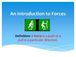
Introduction to forces • We’ve studied motion in one, two, and three dimensions… but what causes motion? • This causality was first understood in the late 1600s by Sir Isaac Newton. • Newton formulated three laws governing moving objects, which we call Newton’s laws of motion. • Newton’s laws were deduced from huge amounts of experimental evidence. • The laws are simple to state but intricate in their application.

What are some properties of a force?

There are four common types of forces • The normalforce: When an object pushes on a surface, the surface pushes back on the object perpendicular to the surface. This is a contact force. • Friction force: This force occurs when a surface resists sliding of an object and is parallel to the surface. Friction is a contact force.

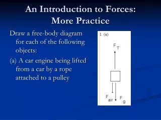
There are four common types of forces II • Tension force:A pulling force exerted on an object by a rope or cord. This is a contact force. • Weight: The pull of gravity on an object. This is a long-range force.

What are the magnitudes of common forces?

Drawing force vectors—Figure 4.3 • Use a vector arrow to indicate the magnitude and direction of the force.

Superposition of forces—Figure 4.4 • Several forces acting at a point on an object have the same effect as their vector sum acting at the same point.

Decomposing a force into its component vectors • Choose perpendicular x and y axes. • Fx and Fyare the components of a force along these axes. • Use trigonometry to find these force components.

Notation for the vector sum—Figure 4.7 • The vector sum of all the forces on an object is called the resultant of the forces or the net forces.

Superposition of forces—Example 4.1 • Force vectors are most easily added using components: Rx = F1x + F2x + F3x + … , Ry = F1y + F2y + F3y + … . See Example 4.1 (which has three forces).

Introduction Forces