Download
1 / 21
210 likes | 300 Views
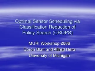
Optimal Sensor Scheduling via Classification Reduction of Policy Search (CROPS). MURI Workshop 2006 Doron Blatt and Alfred Hero University of Michigan. Motivating Example: Landmine Confirmation/Detection. EMI. GPR. Seismic.

E N D
Optimal Sensor Scheduling via Classification Reduction ofPolicy Search (CROPS) MURI Workshop 2006 Doron Blatt and Alfred Hero University of Michigan
Motivating Example: Landmine Confirmation/Detection EMI GPR Seismic • A vehicle carries three sensors for land-mine detection, each with its own characteristics. • The goal is to optimally schedule the three sensors for mine detection. • This is a sequential choice of experiment problem (DeGroot 1970). • Optimal policy maximizes average reward Rock Nail Plastic Anti-personnel Mine Plastic Anti-tank Mine New location EMI Seismic GPR EMI data GPR data Seismic data EMI Seismic EMI data Final detection Seismic data Seismic data Final detection Final detection
Reinforcement Learning • General objective: To find optimal policies for controlling stochastic decision processes: • without an explicit model. • when the exact solution is intractable. • Applications: • Sensor scheduling. • Treatment design. • Elevator dispatching. • Robotics. • Electric power system control. • Job-shop Scheduling.
Learning from Generative Models • It is possible to evaluate the value of any policy from trajectory trees: • Let be the sum of rewards on the path that agrees with policy on the ith tree. Then, O0 a0=0 a0=1 O10 O11 a1=0 a1=1 a1=0 a1=1 O200 O201 O210 O211 a2=0 a2=1 a2=0 a2=1 a2=0 a2=1 a2=0 a2=1 O3000 O3001 O3010 O3011 O3100 O3101 O3110 O3111
Three sources of error in RL • Coupling of optimal decisions at each stage: finding the optimal decision rule at a certain stage hinges on knowing the optimal decision rule for future stages • Misallocation of approximation resources to state space: without knowing the optimal policy one cannot sample from the distribution that it induces on the stochastic system’s state space • Inadequate control of generalization errors: without a model ensemble averages must be approximated from training trajectories • J. Bagnell, S. Kakade, A. Ng, and J. Schneider, “Policy search by dynamic programming,” in Advances in Neural Information Processing Systems, vol. 16. 2003. • A. Fern, S. Yoon, and R. Givan, “Approximate policy iteration with a policy language bias,” in Advances in Neural Information Processing Systems, vol. 16, 2003. • M. Lagoudakis and R. Parr, “Reinforcement learning as classification: Leveraging modern classifiers,” in Proceedings of the Twentieth International Conference on Machine Learning, 2003. • J. Langford and B. Zadrozny, “Reducing T-step reinforcement learning to classification,” http://hunch.net/∼jl/projects/reductions/reductions.html, 2003. • M. Kearns, Y. Mansour, and A. Ng, “Approximate planning in large POMDPs via reusable trajectories,” in Advances in Neural Information Processing Systems, vol. 12. MIT Press, 2000. • S. A. Murphy, “A generalization error for Q-learning,” Journal of Machine Learning Research, vol. 6, pp. 1073–1097, 2005.
Learning from Generative Models • Drawbacks: • The combinatorial optimization problem: can only be solved for small n and small . • Our remedies: • Break the multi-stage search problem into a sequence of single-stage optimization problems. • Use a convex surrogate to simplify each optimization problem. • Will obtain generalization bounds similar to (Kearns…,’00) but that apply to the case in which the decision rules are estimated sequentially by reduction to classification
Fitting the Hindsight Path • Zadrozny & Langford 2003: on each tree find the reward maximizing path. • Fit T+1 classifiers to these paths. • Driving the classification error to zero is equivalent to finding the optimal policy. • Drawback: In stochastic problems, no classifier can predict the hindsight action choices. O0 a0=0 a0=1 O10 O11 a1=0 a1=1 a1=0 a1=1 O200 O201 O210 O211 a2=0 a2=1 a2=0 a2=1 a2=0 a2=1 a2=0 a2=1 O3000 O3001 O3010 O3011 O3100 O3101 O3110 O3111
Approximate Dynamic Programming Approach • Assume the policy class has the form: • Estimating T via tree pruning: • This is the empirical equivalent of: • Call the resulting policy O0 a0=0 Choose random actions O10 a1=1 O201 Solve single-stage RL problem a2=0 a2=1 O3010 O3011
Approximate Dynamic Programming Approach O0 • Estimating T-1 given via tree pruning: • This is the empirical equivalent of: a0=0 Choose random actions O10 Solve single-stage RL problem a1=0 a1=1 O200 O201 Propagate rewards according to a2=0 a2=1 O3000 O3011
Approximate Dynamic Programming Approach Propagate rewards according to • Estimating T-2=0 given and via tree pruning: • This is the empirical equivalent of: O0 Solve single-stage RL problem a0=0 a0=1 O10 O11 a1=1 a1=0 O201 O210 a2=1 a2=1 O3011 O3101
O0 a0=-1 a0=1 O1-1 O11 Reduction to Weighted Classification • Our approximate dynamic programming algorithm converts the multi-stage optimization problem into a sequence of single-stage optimization problems. • Unfortunately each sequence is still a combinatorial optimization problem. • Our solution: reduce this to learning classifiers with convex surrogate. • This classification reduction is different from that of Langford&Zarodny:03 • Consider a single-stage RL problem: • Consider a class of real valued functions • Each induces a policy: • Optimal action classifies (Blatt&Hero:NIPS05):
Reduction to Weighted Classification • It is often much easier to solvewhere is a convex function. • For example: • In neural network training is the truncated quadratic loss. • In boosting is the exponential loss. • In support vector machines is the hinge loss. • In logistic regression is the scaled deviance. • The effect of introducing is well understood for the classification problem and the results can be applied to the single-stage RL problem as well.
Reduction to Weighted ClassificationMulti-Stage Problem • Let be the policy estimated by the approximate dynamic programming algorithm, where each single-stage RL problem is solved via minimization. • Theorem 2: Assume P-dim( ) = dt, t=0, …, T. Then, with probability greater than 1-, over the set of trajectory trees,for n satisfying • Proof uses recent results in P. L. Bartlett, M. I. Jordan, and J. D. McAulie, “Convexity, classification, and risk bounds,” Journal of the American Statistical Association, vol. 101, no. 473, pp. 138–156, March 2006. • Tighter than analogous Q-learning bound (Murphy:JMLR2005).
Landsat MSS Experiment • LANDSAT Multispectral Scanner (MSS) • Multispectral scanning radiometer that was carried on board Landsat 1-5. • MSS data consists of four spectral bands: • Visible green • Visible red • Near-infrared 1 • Near-infrared 2 • The resolution for all bands is 79 meters, and the approximate scene size is 185 x 170 kilometers. • STATLOG Project (Michie&etal:94): anotated dataset for testing classifier performance. • Data consists of 4435 training cases and 2000 test cases. • Each case is a 3x3x4 image stack in 36 dimensions having 1 class attribute • There are 6 class labels: • Red soil • Cotton • Vegetation stubble • Gray soil • Damp gray soil • Very damp gray soil • Unequal class sizes in both training and test sets.
Waveform Scheduling: CROPS Bands (1,4) • For each image location we adopt two stage policy to classify its label: • Select one of 6 possible pairs of 4 MSS bands for initial illumination • Based on initial measurement either: • Make final decision on terrain class and stop • Illuminate with remaining two MSS bands and make final decision • Reward is average probability of correct decision minus stopping time (energy) New location Bands (1,2) Bands (1,3) Bands (2,3) Bands (2,4) Bands (3,4) Classify Bands (1,4) Reward=I(correct) Classify Reward=I(correct)-c
Non-myopic is better Myopic is good Best four sensors Best two sensors Optimal sub-band usage under energy constraints
CLT SB Sub-band performance Best myopic choice. Best non-myopic choice when likely to take more than one observation.
Sub-band optimal scheduling • Optimal initial sub-bands are 1+2 * Additional * Classify bands
Alternative Comparisons LANDSAT data: total of 4 bands, each produce a 9 dimensional vector. * C is the cost of using the additional two bands. Best myopic initial pair: (2,3) Non-myopic initial pair: (2,3) Performance with all four bands Performance of all four bands
Conclusions • Elements of CROPS • Gauss-Seidel-type DP approximation reduces multi-stage to sequence of single-stage RL problems • Classification reduction is used to solve each of these signal stage RL problems • Obtained tight finite sample generalization error bounds for RL based on classification theory • CROPS methodology illustrated for energy constrained landmine detection and waveform selection
Publications • Blatt D., “Adaptive Sensing in Uncertain Environments ,” PhD Thesis, Dept EECS, University of Michigan, 2006. • Blatt D. and Hero A. O., "From weighted classification to policy search", Nineteenth Conference on Neural Information Processing Systems (NIPS), 2005. • Kreucher C., Blatt D., Hero A. O., and Kastella K., ``Adaptive multi-modalitysensor scheduling for detection and tracking of smart targets'', Digital Signal Processing, 2005. • Blatt D., Murphy S.A., and Zhu J. "A-learning for Approximate Planning", Technical Report 04-63, The Methodology Center, Pennsylvania State University. 2004.