Download
1 / 1
30 likes | 265 Views
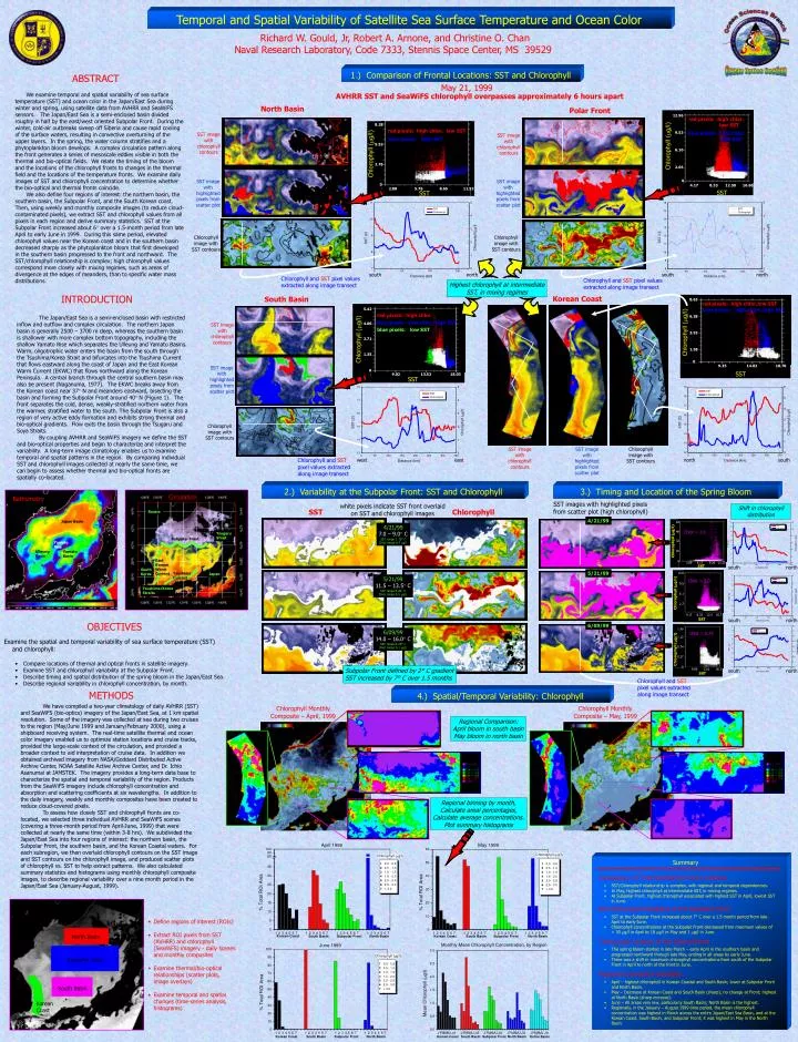
12.96. 9.53. Chlorophyll ( g/l). 6.10. 2.66. 0. 4.17. 8.33. 12.50. 16.66. SST. Circulation. Bathymetry. Russia. Japan Basin. Tsugaru Strait. Subpolar Front. Yamato Rise. Ulleung Basin. Yamato Basin. East Korean Warm Current. South Korea. Tsushima Current. Japan.

E N D
12.96 9.53 Chlorophyll (g/l) 6.10 2.66 0 4.17 8.33 12.50 16.66 SST Circulation Bathymetry Russia Japan Basin Tsugaru Strait Subpolar Front Yamato Rise Ulleung Basin Yamato Basin East Korean Warm Current South Korea Tsushima Current Japan Tsushima/Korea Straits 64 48 32 Chlorophyll (g/l) 16 0 3.09 6.17 9.26 12.35 SST 13.0 9.5 Chlorophyll (g/l) 6.1 2.7 4.17 8.33 12.5 16.7 SST 1.49 1.12 0.74 Chlorophyll (g/l) 0.37 0 9.05 13.6 18.1 SST North Basin Subpolar Front South Basin Korean Coast Temporal and Spatial Variability of Satellite Sea Surface Temperature and Ocean Color Richard W. Gould, Jr, Robert A. Arnone, and Christine O. Chan Naval Research Laboratory, Code 7333, Stennis Space Center, MS 39529 1.) Comparison of Frontal Locations: SST and Chlorophyll ABSTRACT May 21, 1999 We examine temporal and spatial variability of sea surface temperature (SST) and ocean color in the Japan/East Sea during winter and spring, using satellite data from AVHRR and SeaWiFS sensors. The Japan/East Sea is a semi-enclosed basin divided roughly in half by the east/west oriented Subpolar Front. During the winter, cold-air outbreaks sweep off Siberia and cause rapid cooling of the surface waters, resulting in convective overturning of the upper layers. In the spring, the water column stratifies and a phytoplankton bloom develops. A complex circulation pattern along the front generates a series of mesoscale eddies visible in both the thermal and bio-optical fields. We relate the timing of the bloom and the locations of the chlorophyll fronts to changes in the thermal field and the locations of the temperature fronts. We examine daily images of SST and chlorophyll concentration to determine whether the bio-optical and thermal fronts coincide. We also define four regions of interest: the northern basin, the southern basin, the Subpolar Front, and the South Korean coast. Then, using weekly and monthly composite images (to reduce cloud-contaminated pixels), we extract SST and chlorophyll values from all pixels in each region and derive summary statistics. SST at the Subpolar Front increased about 6 over a 1.5-month period from late April to early June in 1999. During this same period, elevated chlorophyll values near the Korean coast and in the southern basin decreased sharply as the phytoplankton bloom that first developed in the southern basin progressed to the front and northward. The SST/chlorophyll relationship is complex; high chlorophyll values correspond more closely with mixing regimes, such as areas of divergence at the edges of meanders, than to specific water mass distributions. AVHRR SST and SeaWiFS chlorophyll overpasses approximately 6 hours apart North Basin Polar Front red pixels: high chlor, low SST 8.28 red pixels: high chlor, low SST blue pixels: high chlor, high SST SST image with chlorophyll contours SST image with chlorophyll contours blue pixels: high SST 5.52 Chlorophyll (g/l) 2.76 SST image with highlighted pixels from scatter plot SST image with highlighted pixels from scatter plot 0 2.88 5.76 8.65 11.53 SST Chlorophyll image with SST contours Chlorophyll image with SST contours south north south north Chlorophyll and SST pixel values extracted along image transect Chlorophyll and SST pixel values extracted along image transect Highest chlorophyll at intermediate SST, in mixing regimes INTRODUCTION Korean Coast South Basin 8.63 red pixels: high chlor,low SST 5.42 blue pixels: high chlor, high SST red pixels: high chlor 6.28 The Japan/East Sea is a semi-enclosed basin with restricted inflow and outflow and complex circulation. The northern Japan basin is generally 2500 – 3700 m deep, whereas the southern basin is shallower with more complex bottom topography, including the shallow Yamato Rise which separates the Ulleung and Yamato Basins. Warm, oligotrophic water enters the basin from the south through the Tsushima/Korea Strait and bifurcates into the Tsushima Current that flows eastward along the coast of Japan and the East Korean Warm Current (EKWC) that flows northward along the Korean Peninsula. A central branch through the central southern basin may also be present (Naganuma, 1977). The EKWC breaks away from the Korean coast near 37 N and meanders eastward, bisecting the basin and forming the Subpolar Front around 40 N (Figure 1). The front separates the cold, dense, weakly-stratified northern water from the warmer, stratified water to the south. The Subpolar Front is also a region of very active eddy formation and exhibits strong thermal and bio-optical gradients. Flow exits the basin through the Tsugaru and Soya Straits. By coupling AVHRR and SeaWiFS imagery we define the SST and bio-optical properties and begin to characterize and interpret the variability. A long-term image climatology enables us to examine temporal and spatial patterns in the region. By comparing individual SST and chlorophyll images collected at nearly the same time, we can begin to assess whether thermal and bio-optical fronts are spatially co-located. blue pixels: low chlor, high SST 4.06 SST image with chlorophyll contours blue pixels: low SST Chlorophyll (g/l) 3.93 Chlorophyll (g/l) 2.71 1.58 1.35 0 9.35 14.02 18.70 SST image with highlighted pixels from scatter plot 0 SST 9.02 13.52 18.03 SST Chlorophyll image with SST contours SST image with chlorophyll contours SST image with highlighted pixels from scatter plot Chlorophyll image with SST contours Chlorophyll and SST pixel values extracted along image transect west east north south 2.) Variability at the Subpolar Front: SST and Chlorophyll 3.) Timing and Location of the Spring Bloom SST images with highlighted pixels from scatter plot (high chlorophyll) white pixels indicate SST front overlaid on SST and chlorophyll images Shift in chlorophyll distribution SST Chlorophyll 4/21/99 4/21/99 7.0 – 9.0 C SST range 1-15° C Chlor range 0-7 g/l Chlor > 2.0 south north 5/21/99 5/21/99 11.5 – 13.5 C SST range 5-20° C Chlor range 0-5 g/l Chlor > 2.0 south north OBJECTIVES 6/09/99 6/09/99 14.0 – 16.0 C SST range 8-20° C Chlor range 0-1 g/l Chlor > 0.75 • Examine the spatial and temporal variability of sea surface temperature (SST) and chlorophyll: • Compare locations of thermal and optical fronts in satellite imagery. • Examine SST and chlorophyll variability at the Subpolar Front. • Describe timing and spatial distribution of the spring bloom in the Japan/East Sea. • Describe regional variability in chlorophyll concentration, by month. Subpolar Front defined by 2° C gradient SST increased by 7° C over 1.5 months south north Chlorophyll and SST pixel values extracted along image transect METHODS 4.) Spatial/Temporal Variability: Chlorophyll We have compiled a two-year climatology of daily AVHRR (SST) and SeaWiFS (bio-optics) imagery of the Japan/East Sea, at 1 km spatial resolution. Some of the imagery was collected at sea during two cruises to the region (May/June 1999 and January/February 2000), using a shipboard receiving system. The real-time satellite thermal and ocean color imagery enabled us to optimize station locations and cruise tracks, provided the large-scale context of the circulation, and provided a broader context to aid interpretation of cruise data. In addition we obtained archived imagery from NASA/Goddard Distributed Active Archive Center, NOAA Satellite Active Archive Center, and Dr. Ichio Asanumai at JAMSTEK. The imagery provides a long-term data base to characterize the spatial and temporal variability of the region. Products from the SeaWiFS imagery include chlorophyll concentration and absorption and scattering coefficients at six wavelengths. In addition to the daily imagery, weekly and monthly composites have been created to reduce cloud-covered pixels. To assess how closely SST and chlorophyll fronts are co-located, we selected three individual AVHRR and SeaWiFS scenes (covering a three-month period from April-June, 1999) that were collected at nearly the same time (within 3-8 hrs). We subdivided the Japan/East Sea into four regions of interest: the northern basin, the Subpolar Front, the southern basin, and the Korean Coastal waters. For each subregion, we then overlaid chlorophyll contours on the SST image and SST contours on the chlorophyll image, and produced scatter plots of chlorophyll vs. SST to help extract patterns. We also calculated summary statistics and histograms using monthly chlorophyll composite images, to describe regional variability over a nine month period in the Japan/East Sea (January-August, 1999). Chlorophyll Monthly Composite – April, 1999 Chlorophyll Monthly Composite – May, 1999 Regional Comparison: April bloom in south basin May bloom in north basin Regional binning by month, Calculate areal percentages, Calculate average concentrations. Plot summary histograms Summary Comparison of Thermal/Optical Front Locations • SST/Chlorophyll relationship is complex, with regional and temporal dependencies. • In May, highest chlorophyll at intermediate SST, in mixing regimes. • At Subpolar Front, highest chlorophyll associated with highest SST in April, lowest SST in June. SST/Chlorophyll Variability at the Subpolar Front • SST at the Subpolar Front increased about 7° C over a 1.5 month period from late-April to early-June. • Chlorophyll concentrations at the Subpolar Front decreased from maximum values of > 30 g/l in April to 10 g/l in May and 1 g/l in June. • Define regions of interest (ROIs) • Extract ROI pixels from SST (AVHRR) and chlorophyll (SeaWiFS) imagery - daily scenes and monthly composites • Examine thermal/bio-optical relationships (scatter plots, image overlays) • Examine temporal and spatial changes (time-series analysis, histograms) Timing and Location of the Spring Bloom • The spring bloom started in late March – early April in the southern basin and progressed northward through late May, ending in all areas by early June. • There was a shift in maximum chlorophyll concentrations from south of the Subpolar Front in April to north of the front in June. Regional Chlorophyll Variability • April – highest chlorophyll in Korean Coastal and South Basin; lower at Subpolar Front and North Basin. • May – Decrease at Korean Coast and South Basin (sharp); no change at Front; highest at North Basin (sharp increase). • June – All areas very low, particularly South Basin; North Basin is the highest. • Regionally, in the January – August 1999 time period, the mean chlorophyll concentration was highest in March across the entire Japan/East Sea Basin, and at the Korean Coast, South Basin, and Subpolar Front; it was highest in May in the North Basin.