Download
1 / 30
300 likes | 444 Views
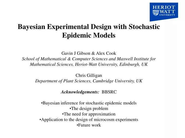
Bayesian Experimental Design with Stochastic Epidemic Models Gavin J Gibson & Alex Cook School of Mathematical & Computer Sciences and Maxwell Institute for Mathematical Sciences, Heriot-Watt University, Edinburgh, UK Chris Gilligan Department of Plant Sciences, Cambridge University, UK

E N D
Bayesian Experimental Design with Stochastic Epidemic Models • Gavin J Gibson & Alex Cook • School of Mathematical & Computer Sciences and Maxwell Institute for Mathematical Sciences, Heriot-Watt University, Edinburgh, UK • Chris Gilligan • Department of Plant Sciences, Cambridge University, UK • Acknowledgements: BBSRC • Bayesian inference for stochastic epidemic models • The design problem • The need for approximation • Application to the design of microcosm experiments • Future work
History of individual i. time S E I R ? ? ? ? susceptible exposed infective removed Epidemics: Observable and unobservable processes Consider SEIR model for an epidemic in a closed population that mixes homogeneously. Diagnostic tests: • Limited frequency of tests • Certain states indistinguishable (e.g. S & E) • False negative and positive results
Stochastic model: S E: If j is in state S at time t, then Pr(j is exposed in (t, t+dt)) = bI(t)dt E I: (random time in E) I R: (random time in I) Parameters: q = (b, qE, qI) How can we estimate the parameters from the observations?
Likelihood and Bayesian inference in a nutshell… Given observations y (from model M with unknown parameters, q) likelihood principle says all evidence about q contained in likelihood L(q|y) = Pr(y|q) “the probability of the observations given q”. Bayesian approach. Represent prior beliefs re q as density p(q). Update in light of y using Bayes’ Theorem p(q|y) p(q)L(q|y). When q multivariate, inference on individual components made using marginal posterior density.
Bayesian inference for epidemic models • Let y represent observed data (incomplete), z represent complete data (times and nature of all events). • Problem is that Pr(z|q) usually tractable, but • Solution: Consider ‘hidden’ aspects, x, of the data as additional unknown parameters. Investigate the joint posterior density p(q, x |y). Make inference on q by marginalisation. • Now, by Bayes’ Theorem • p(q, x |y) p(q)p(x, y|q) Integrate over all z consistent with y Likelihood for augmented data (tractable)
Using Markov chain methods we cangenerate samples {(qi, xi)} from p(q, x|y), where p(q, x |y) p(q)p(x, y|q) Construct Markov chain with this stationary distribution which iterates by proposing & accepting/rejecting changes to the current state (qi, xi) to obtain (qi+1, xi+1). Updates to (some components of) q can often be carried out by Gibb’s steps. Updates to x, usually requires M-H and RJ type approaches. Algorithms of this type have been developed and applied to the analysis of data (see e.g. GJG (1997), GJG & ER (1998, 2001), GS & GJG (2004a, 2004b), O’Neill & Roberts (1999), O’Neill & Becker (2001), Forrester et al. (2006))
Example. Epidemics of R solani in radish (with Plant Sciences, Cambridge) Population size 50 (with and without added T. viride). No Trichoderma Trichoderma added
A simple model for this is the SEI with primary, secondary infection + quenching (Gibson et al., PNAS, 2004) For any susceptible individual at time t, the probability of becoming exposed in the time interval [t, t+dt) is given by R(t) = (rp + rsI(t))exp{-at}. Exposed individuals become infectious at fixed time m after exposure. Using vague uniform priors over finite windows we obtain the following posteriors for the model parameters, suggesting that Trichodermaacts on primary infection process.
SECONDARY (rs) PRIMARY (rp) QUENCHING (a) LATENT PERIOD (m)
Statisticians (like me) have tended to focus on analyses of particular data sets, often historical to illustrate the value of the Bayesian approach. Emphasis placed on tackling the complexity arising from partial observation and the need to respect the likelihood principle. Experimental design requires us to address the uncertainty in future realisations of a process and the range of ways in which it could be observed. To address these two sources of complexity simultaneously in the context of epidemic models (stochastic, spatial, nonlinear) is a major challenge.
Experimental design with stochastic epidemic models: Propose to use Bayesian framework (Muller et al., 1999) for identifying optimal designs. q ~ p(q) represents current belief regarding q. z ~ p(z | q) – ‘complete’ future realisation of process. d(z ) – censored/filtered version of z arising from design d chosen from some suitable space of designs. U(d(z )) utility function quantifying information in d(z), and or cost of the experiment. Aim: Select d to maximise the expectation of U(d(z ))
Identifying optimal designs ‘Trick’ is to treat the design, d, as an additional variable and assign joint distribution to (q, z, d) so that the joint density is, f(q, z, d) p(q)p(z|q)U(d(z)) Integrating w.r.t.z, we obtain f(d|q) E(U(d)|q), the expectation of U conditional on q. Integrating with respect to q we find that f(d) E(U(d)). Hence, identifying the optimal design for future experiment given current belief re q is equivalent to identifying the mode of f(d).In theory we could investigate f using MCMC methods.
Looks simple – where do the difficulties arise? If you’re a Bayesian then you should base your utility on the posterior density you obtain in an experiment. One sensible(?) measure would be Kullback-Leibler divergence between prior and posterior. Let y = d(z) Then U(d(z)) = However, the posterior p(q|y) is usually difficult to obtain. Therefore we will have to use approximations to it. Go back to the R solani system. May be nasty!
Example. Epidemics of R solani in radish (with Plant Sciences, Cambridge)
I(t) t3 t2 t1 Let’s look at problem of selecting a sparse set of m observation times for microcosm experiments. We focus on a simpler model in which the latent period is assumed to be zero. e.g. m = 3 For this experiment y = (I(t1), I(t2), I(t3)), q = (rp, rs, a). We wish to approximate
First approximation: Approximate the prior with a discrete uniform prior by drawing a random sample from p. Second approximation: Approximate the likelihood L(q) using moment-closure methods (e.g. Krishnarajah et al., 2005) Basic idea: L(q) = P(I(t1) = y1|q)×P(I(t2) = y2 | I(t1) = y1, q) × P(I(tk) = yk | I(tk-1) = yk-1,q) ……. Approximate each term individually using moment-closure. First suppose a = 0. Now, for t > tk, let n0 = N – I(tk), C = rp + rsI(tk), J(t) = I(t) – I(tk). Remaining susceptibles Effective primary infection rate Infections after tk
Idea of MC is to approximate the evolution of moments of population variables by a system of differential equations. For our simple model: Pr(J(t+dt) – J(t) = 1) = (C(n0-J(t)) + rsJ(t)(n0-J(t))dt = {Cn0 + ( rsn0 - C)J(t) – rsJ2(t)}dt E(J(t)) = Cn0 + (rsn0 - C)E(J(t)) – rsE(J2(t)) This equation involves the 2nd moment of J(t).
Pr(J2(t+dt) – J2(t) = 2J(t) + 1) = (C(n0-J(t)) + rsJ(t)(n0-J(t))dt • = {Cn0 + ( rsn0 - C)J(t) – rsJ2(t)}dt • E(J(t+dt)-J(t)|J(t)) = (2J(t) + 1){Cn0 + (rsn0 - C)E(J(t)) – rsE(J2(t)}dt E(J2(t)) = Cn0 + (rsn0 + 2Cn0 – C)E(J(t)) - (2n0rs – rs -2C)E(J2(t)) – 2CE(J3(t)) Unfortunately, 3rd moment appears on r.h.s.! In general, equation for kth moment includes terms in (k+1)th moment.
Solution: Close the system of equations by assuming that J(t) has a particular distribution. Here we assume that J(t) ~ BetaBin(n0, a(t), b(t)). a(t) and b(t) are determined by the first two moments. E(J3(t)) is then a function of a(t) and b(t), and hence the first two moments. Substituting this function into the differential equation for E(J2(t)) allows the system to be closed and solved using Euler’s method. Previous work (Krishnarajah et al., BMB 2005) indicates that the BetaBin distribution provides a good approximation to the distribution of J(t).
Comparison of moment-closure with exact probability function. No Trichoderma Trichoderma t = 1 t = 5 t = 15
Estimating L(rp, rs, a) I(t3) I(t) I(t2) L = p1p2p3 I(t1) t1 t2 t3 Integrate ODE to get distribution for I(t1), given I(0) = 0. Integrate ODE to get distribution for I(t2), given I(t1). Integrate ODE to get distribution for I(t3), I(t2).
Full algorithm for experimental design Recall we wish to draw from joint density f(q, z, d) p(q)p(z|q)U(d(z)) where d represents a set of m distinct sampling times arranged between t = 0 and tmax. q = (rp, rs, a) and is a priori uniform over a finite set of points (random sample from continuous p). z represents complete process and comprises the infection times for all individuals in the population.
Outline of steps for updating (qi, zi, di) • Propose new (q′, z′) by drawing q′ from the prior and simulating realisation z′ from the model. • Accept with probability min{1, U(di(z′))/U(di(zi))}, otherwise reject. • Propose changes to sampling times e.g. using M-H methods. Proposed d′ can be di with perturbation applied to one of sampling times. t1 t2 tj tm di d′ Accept with prob. min{1, U(d′(zi+1))/U(di(zi+1))}
Note: • The algorithm identifies optimal design for a single-replicate experiment. Optimal designs for multi-replicate experiments look broadly similar. • The utility can be ‘sharpened’ by adapting the algorithm to propose k independent (q, z) combinations. Now f(d) [E(U(d(z))]k. We illustrate some optimal designs for the unquenched SI model. (See Cook et al., in prep.)
Now a more practically relevant situation – designing experiments for the R solani system (without Trichoderma). rp rs a Sample from joint posterior gives new prior, p′.
We consider 2 situations: Progressive design: How should you repeat experiment to maximise expected information change w.r.t. p′? (Uses p′ to propose new z’s and p′ as prior in utility calculation.) Confirmatory (pedagogic) design: How should you repeat experiment to maximise expected information change w.r.t. p? (Uses p′ to propose new z’s and p as prior in utility calculation.) Designs constrained to be subset of sampling times in original experiment.
pedagogic rp progressive rs a Results: Designs and their application to analysis of original data. Posteriors shown are for pedagogic designs.
Further work: • Designs for imperfect diagnostic tests • Adaptive designs • Extension to spatio-temporal modelling – designs include location of host or inoculum. • Non-Markovian systems. • Efficient approximation of intractable likelihoods is key to all of these problems.