Download
1 / 20
210 likes | 358 Views
Sorting and Selection. 1, c. 3, a. 3, b. 7, d. 7, g. 7, e. . . . . . . . 0. 1. 2. 3. 4. 5. 6. 7. 8. 9. B. Lower Bounds. Lower bound : an estimate on a minimum amount of work needed to solve a given problem Examples:

E N D
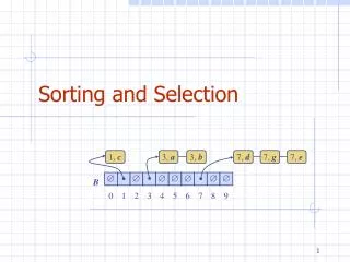
Sorting and Selection 1, c 3, a 3, b 7, d 7, g 7, e 0 1 2 3 4 5 6 7 8 9 B
Lower Bounds Lower bound: an estimate on a minimum amount of work needed to solve a given problem Examples: • number of comparisons needed to find the largest element in a set of n numbers • number of comparisons needed to sort an array of size n • number of comparisons necessary for searching in a sorted array
Lower Bounds (cont.) • Lower bound can be • an exact count • an efficiency class () • Tight lower bound: there exists an algorithm with the same efficiency as the lower bound Problem Lower bound Tightness sorting (comparison-based) (nlog n) yes searching in a sorted array (log n) yes element uniqueness (nlog n) yes n-digit integer multiplication (n) unknown multiplication of n-by-n matrices (n2) unknown
Decision Trees Decision tree — a convenient model of algorithms involving comparisons in which: • internal nodes represent comparisons • leaves represent outcomes (or input cases) Decision tree for 3-element insertion sort
Decision Trees and Sorting Algorithms • Any comparison-based sorting algorithm can be represented by a decision tree (for each fixed n) • Number of leaves (outcomes) n! • Height of binary tree with n! leaves log2n! • Minimum number of comparisons in the worst case log2n! for any comparison-based sorting algorithm, since the longest path represents the worst case and its length is the height • log2n! n log2n (by Sterling approximation) • This lower bound is tight (mergesort or heapsort) Ex. Prove that 5 (or 7) comparisons are necessary and sufficient for sorting 4 keys (or 5 keys, respectively).
Let be S be a sequence of n (key, element) items with keys in the range [0, N- 1] Bucket-sort uses the keys as indices into an auxiliary array B of sequences (buckets) Phase 1: Empty sequence S by moving each item (k, o) into its bucket B[k] Phase 2: For i = 0, …,N -1, move the items of bucket B[i] to the end of sequence S Analysis: Phase 1 takes O(n) time Phase 2 takes O(n+ N) time Bucket-sort takes O(n+ N) time Bucket-Sort AlgorithmbucketSort(S,N) Inputsequence S of (key, element) items with keys in the range [0, N- 1]Outputsequence S sorted by increasing keys B array of N empty sequences whileS.isEmpty() f S.first() (k, o) S.remove(f) B[k].insertLast((k, o)) for i 0 toN -1 whileB[i].isEmpty() f B[i].first() (k, o) B[i].remove(f) S.insertLast((k, o))
7, d 1, c 3, a 7, g 3, b 7, e 1, c 3, a 3, b 7, d 7, g 7, e B 0 1 2 3 4 5 6 7 8 9 1, c 3, a 3, b 7, d 7, g 7, e Example • Key range [0, 9] Phase 1 Phase 2
Key-type Property The keys are used as indices into an array and cannot be arbitrary objects No external comparator Stable Sort Property The relative order of any two items with the same key is preserved after the execution of the algorithm Extensions Integer keys in the range [a, b] Put item (k, o) into bucketB[k - a] String keys from a set D of possible strings, where D has constant size (e.g., names of the 50 U.S. states) Sort D and compute the rank r(k)of each string k of D in the sorted sequence Put item (k, o) into bucket B[r(k)] Properties and Extensions
Lexicographic Order • A d-tuple is a sequence of d keys (k1, k2, …, kd), where key ki is said to be the i-th dimension of the tuple • Example: • The Cartesian coordinates of a point in space are a 3-tuple • The lexicographic order of two d-tuples is recursively defined as follows (x1, x2, …, xd) < (y1, y2, …, yd)x1 <y1 x1=y1 (x2, …, xd) < (y2, …, yd) I.e., the tuples are compared by the first dimension, then by the second dimension, etc.
Lexicographic-Sort AlgorithmlexicographicSort(S) Inputsequence S of d-tuplesOutputsequence S sorted in lexicographic order for i ddownto 1 stableSort(S, Ci) • Let Ci be the comparator that compares two tuples by their i-th dimension • Let stableSort(S, C) be a stable sorting algorithm that uses comparator C • Lexicographic-sort sorts a sequence of d-tuples in lexicographic order by executing d times algorithm stableSort, one per dimension • Lexicographic-sort runs in O(dT(n)) time, where T(n) is the running time of stableSort Example: (7,4,6) (5,1,5) (2,4,6) (2, 1, 4) (3, 2, 4) (2, 1, 4) (3, 2, 4) (5,1,5) (7,4,6) (2,4,6) (2, 1, 4) (5,1,5) (3, 2, 4) (7,4,6) (2,4,6) (2, 1, 4) (2,4,6) (3, 2, 4) (5,1,5) (7,4,6)
Radix-sort is a specialization of lexicographic-sort that uses bucket-sort as the stable sorting algorithm in each dimension Radix-sort is applicable to tuples where the keys in each dimension i are integers in the range [0, N- 1] Radix-sort runs in time O(d( n+ N)) Radix-Sort AlgorithmradixSort(S, N) Inputsequence S of d-tuples such that (0, …, 0) (x1, …, xd) and (x1, …, xd) (N- 1, …, N- 1) for each tuple (x1, …, xd) in SOutputsequence S sorted in lexicographic order for i ddownto 1 bucketSort(S, N)
Radix-Sort for Binary Numbers • Consider a sequence of nb-bit integers x=xb- 1 … x1x0 • We represent each element as a b-tuple of integers in the range [0, 1] and apply radix-sort with N= 2 • This application of the radix-sort algorithm runs in O(bn) time • For example, we can sort a sequence of 32-bit integers in linear time AlgorithmbinaryRadixSort(S) Inputsequence S of b-bit integers Outputsequence S sorted replace each element x of S with the item (0, x) for i 0 tob - 1 replace the key k of each item (k, x) of S with bit xi of x bucketSort(S, 2)
1001 0001 1001 1001 0010 1101 0010 0001 0010 1110 0010 0001 1001 1101 1001 1101 1101 0001 0010 1101 1110 1110 1110 1110 0001 Example • Sorting a sequence of 4-bit integers
Order Statistics • The ith order statistic in a set of n elements is the ith smallest element • The minimumis thus the 1st order statistic • The maximum is (duh)the nth order statistic • The median is the n/2 order statistic • If n is even, there are 2 medians • Could calculate order statistics by sorting • Time: O(n lg n) w/ comparison sort • We can do better
Selection Problem • Theselection problem: find the ith smallest element of a set • Two algorithms: • A practical randomized algorithm with O(n) expected running time • A cool algorithm of theoretical interest only with O(n) worst-case running time
Randomized Selection • Key idea: use partition() from quicksort • But, only need to examine one subarray • This saving shows up in running time: O(n) A[q] A[q] q p r
Randomized Selection RandomizedSelect(A, p, r, i) if (p == r) then return A[p]; q = RandomizedPartition(A, p, r) k = q - p + 1; if (i == k) then return A[q]; if (i < k) then return RandomizedSelect(A, p, q-1, i); else return RandomizedSelect(A, q+1, r, i-k); k A[q] A[q] q p r
Review: Randomized Selection • Average case • For upper bound, assume ith element always falls in larger side of partition: • We then showed that T(n) = O(n) by substitution
Linear-Time Median Selection • Given a “black box” O(n) median algorithm, what can we do? • ith order statistic: • Find median x • Partition input around x • if (i (n+1)/2) recursively find ith element of first half • else find (i - (n+1)/2)th element in second half • T(n) = T(n/2) + O(n) = O(n) • Can you think of an application to sorting?
Linear-Time Median Selection • Worst-case O(n lg n) quicksort • Find median x and partition around it • Recursively quicksort two halves • T(n) = 2T(n/2) + O(n) = O(n lg n)