Download
1 / 72
740 likes | 932 Views
Stochastic modeling of flow and transport in highly heterogeneous porous formations Gedeon Dagan Tel Aviv University, Israel Aldo Fiori Università di Roma Tre, Italy. Special Semester on Multiscale Simulation & Analysis in Energy and the Environment Linz, October 3-December 16, 2011

E N D
Stochastic modeling of flow and transport in highly heterogeneous porous formations Gedeon Dagan Tel Aviv University, Israel Aldo Fiori Università di Roma Tre, Italy Special Semester onMultiscale Simulation & Analysis in Energy and the Environment Linz, October 3-December 16, 2011 Numerical Analysis of Multiscale Problems & Stochastic Modelling
The local equations of flow and transport: General definitions • We consider water flow and solute transport through porous media. • A porous medium is an interconnected network of voids (pores) in a solid material • The characteristic length scale d is the pore size: from μm to mm. • The interest is generally in porous bodies of scale L>>d.
Scales • Flow and transport at the pore scale (microscopic scale) are complex due to the geometry (even for artificial media, e.g. mixture of small spheres of equal diameter) • The problem is simplified by defining macroscopic variables: averaging over volumes of scale ℓ, justified by the hierarchy d<<ℓ<<L.
Basic properties • The simplest property is the porosity n=(Volume voids)/(Total volume), n<1 • In a similar manner macroscopic variables: • q - specific discharge (fluid discharge/area of medium) • V=q/n - pore velocity • p - pore pressure • H=(p/(ρg))+z - head (ρ is density, z is elevation) • C - solute concentration (mass of solute/volume of fluid)
Macroscopic scale • Macroscopic variables constitute continuous space fields: the porous medium is replaced by a continuum. • Value of variable at a point x: average over a volume (area) of scale ℓ whose centroid is at x. • Homogeneous medium: no change with x. • Nonhomogeneous medium: slowly varying (scale >>ℓ).
Flow • Experimental determination of flow and transport equations: a laboratory column or a sample (core) of scale L>ℓ.
Flow equations • Darcy's law: • K : hydraulic conductivity (permeability). In nature: 10⁻¹≲K(cm/sec)≲10⁻⁶ • Generalization for 3D flow in space • For incompressible matrix and fluid, conservation of mass
Flow equations (cont.) • Elimination of q leads to • For homogeneous media • General problem of steady flow: given a space domain Ω, given K(x), given boundary conditions H or qnormal on boundary ∂Ω, determine H(x) satisfying flow equation for x∈Ω. Subsequently: q(x)=-K∇H, V(x)=q/n.
Solute transport • At t=0 a conservative solute (tracer) at constant concentration C₀ is inserted at the column entrance x=0; water flows at constant velocity U=q/n. • The BTC (breakthrough curve) at the outlet C(L,t) has an inverse Gaussian shape. C(x,t) obeys the ADE (advective dispersion equation) of solute mass conservation
Solute transport • The solute flux is made up from the advective component UC and the dispersive one • : localpore scale dispersionlongitudinalcoefficient. ForPe>>1 (Pe=Ud/D0, with D0moleculardiffusioncoefficient O(10⁻⁴ cm²/sec) • Dd,0<D0: effectivecoefficientofmoleculardiffusion; αd,L:pore scale longitudinal dispersivity O(d). • ForPe>10: αd,LU>>Dd,0→ mixing due tomicroscopicvelocityvariationsoverridesmoleculardiffusion.
Solute transport • Generalization for transport in space • Dd is the pore scale dispersion tensor. Its principal axes are in the direction of V (longitudinal Dd,L=Dd,0+αd,LU) and normal to V (transversal Dd,T=Dd,0+αd,TU) →Dd(Dd,L,Dd,T,Dd,T). • Generally αd,T<<αd,L (~1/40). If solute is reactive (decay, sorption) a source term has to be added.
General problem of transport • Given a space domain Ω, given the velocity field V(x) solution of the flow problem, given αd,L and αd,T, given initial and boundary conditions for C (e.g. instantaneous or continuous injection in a subdomain of Ω), determine C(x,t) satisfying the transport equation. • Simple case: instantaneous injection of a fluid body of constant concentration C₀ at t=0 in a spherical domain, for constant U. The centroid of the solute body moves with U, and surfaces of constant C are elongated ellipsoids.
Heterogeneity of natural formations • Natural formations (aquifers, petroleum reservoirs) are characterized by scales L =O(10¹-10³meters). Their properties vary in space over scales I much larger than the laboratory scale ℓ. • The hierarchy L>>I>>ℓ>>d is assumed to prevail.
Heterogeneity: Hydraulic conductivity • The property of highest spatial variability is K, which may vary by orders of magnitude in the same formation. It is irregular (seemingly erratic) and generally subjected to uncertainty due to scarcity of data. Conductivity distribution in a cross section of the Borden Site aquifer in Canada (lines of constant –lnK, cm/sec)
Heterogeneity as a random property • K(x), or equivalently Y=lnK, is modeled in statistical terms as RSF (random space function). • The actual formation is regarded as a realization of an ensemble of replicates of same statistical properties. • The ensemble is a convenient mathematical construction to tackle variability and uncertainty. Replicates can be generated numerically by Monte Carlo simulations.
Statistical characterization of hydraulic conductivity • The statisticalstructureof the RSF Y(x) can bequantifiedby the joint PDF (probability density function) ofitsvalues at anarbitrary set ofpointsYi=Y(xi): f(Y1,Y2,…,YN). In turn byvariousmoments • In manyformations the univariate f(Y) wasfoundtofit a normaldistribution where Y’=Y-<Y>, <Y(x)> ensemble mean, σY²is the variance.
Statistical characterization (cont.) • The bivariate f(Y1,Y2) is characterized at second order by the means, the variances and the two-point covariance CY(x₁,x₂)=〈Y′(x₁)Y′(x₂)〉. • If Y is bivariate normal, it is completely defined by these moments. • Stationary RSF: • 〈Y(x)〉=const, σY²=const • CY(x₁,x₂)=σY²ρY(r) (r=x₁-x₂). Isotropic: ρY(r), r=|r| • Integral scale: Anisotropic:
Statistical characterization (cont.) • Common examples of isotropic • Anisotropic: • For axisymmetric anisotropy Ix=Iy and f=Iz/Ix=Ivertical/Ihorizontal is the anisotropy ratio, generally f<1. At second order and for an adopted PDF, the statistical structure is characterized by the parameters:
Ergodic hypothesis • If the length scale L of Ω, L >>I, ensemble averaging can be exchanged with space averaging, e.g. • Since only one realization of formation is available, the hypothesis is generally adopted and identification of statistical structure is carried out by using spatial data of the given formation. • Due to scarcity of data and ergodic limitations practically only the hystogram i.e. f(Y)→〈Y〉,σY² and the covariance can be identified. If it is assumed that Y(xi) is multi-Gaussian, this information is complete.
Stochastic modeling of flow and transport in natural formations • Since the flow equation ∇²H+∇H.∇Y=0 contains the RSF Y, it is a stochastic equation. • The variables H(x,t),q(x,t),V(x,t),C(x,t) are RSF and are defined by the joint PDF of their values at different x and t • The general problem of stochastic modeling: given a space domain Ω, given the RSF Y(x) i.e. K(x), given n, αd,L, αd,T (generally assumed constant), given initial and boundary conditions for H and for C, determine the RSF H,V by solving first the flow equation and subsequently the RSF C(x,t) satisfying the transport equation.
Solutions: numerical Monte Carlo • The conceptually simple and most general approach is by Monte Carlo simulations: realizations of Y are generated, the deterministic equations for each realizations are solved M times, and the complete statistics is determined at N points. • It is computationally extremely demanding and does not lead to insight. At present and for highly heterogeneous formations, they are numerical experiments at most.
Solutions: approximate analytical • We proceed with approximate solutions for the following simplified conditions: • stationary • unbounded domain Ω (i.e. x is far from the boundary) • steady flow, uniform in the mean 〈V〉=U=const (caused by a uniform mean head gradient ∇〈H〉=-J applied on the boundary approximately valid for natural gradient flow)
Solutions: approximate analytical (cont) • After solving for V, transport equation is solved by assuming: • a conservative solute at low concentration • the solute initial condition is of instantaneous injection of a plume at constant C₀ in a volume V₀ or an injection plane normal to the mean flow on an area A₀ • the length scale of V₀ or A₀ are much larger than the integral scale of Y in the transverse direction This idealized scenario may be applied after adaptation to actual formations for natural gradient flows, which are slowly varying in space. In contrast, highly nonuniform flows caused by pumping or injecting wells are more complex.
Impact of heterogeneity on transport: a few examples • Heterogeneity of K(x) has a major effect on transport, which is enhanced by orders of magnitude as compared to local pore scale dispersion. Isoconcentration lines for the Borden experiment
Lagrangean approach and quantification of transport • The initial solute body is regarded as made up from indivisible particles of mass ΔM. In the case of injection in a volume in the resident mode ΔM=C₀ΔV₀. For instantaneous injection in a plane ΔM/M₀ =m₀ ΔA₀ where M₀ is total mass and m₀ is (relative mass of solute)/area, i.e. ∫A₀m₀dA₀ =1 • In the resident mode m₀=const, in the flux proportional mode m₀(a)=[Vx(a)/U](ΔM/M₀ ΔA₀ ) where x=a is a coordinate in A₀ or V₀.
Trajectory definition • x=Xt(t,a) is the trajectory of a particle originating at x=a at t=0 • The solute body at time t is made up from the ensemble of particles at Xt(t,a) • w is the Lagrangean fluid velocity w(t,a)=V[Xt(t,a)], wd is a Wiener or Brownian motion diffusive velocity associated with local scale dispersion
Solution for Lagrangean trajectories • Since the flow solution provides the Eulerian velocity V(x), Xt satisfies the stochastic integral equation • In the numerical approach known as particle tracking it becomes Xt(t+Δt,a)- Xt(t,a)=V[Xt(t,a)]Δt+ΔXd where ΔXd are random independent diffusive displacements associated with local dispersion. If local dispersion is neglected dX/dt=V[X(t,a)] is the trajectory of a fluid particle.
Quantification of plume transport • Here we focus on the global measure of mass arrival at a CP (control plane) at x, normal to the mean flow direction U(U,0,0) with A₀ at x=ax=0 • With M(x,t) the mass of solute which has crossed the CP at time t, m(x,t)=M/M₀ is known as the BTC (m>m(x,0)=0, m<m(x,∞)=1) • From the definition of Xt(t,a) which connects the BTC with the trajectories
Analysis of transport by Breakthrough Curves (BTC) (cont.)
Analysis of transport by Breakthrough Curves (BTC) • It is advantageous to rewrite the problem in terms of the travel time τt(x,a), the time for which the particle has crossed the CP which is related to Xt by x-Xt(τt,a)=0, i.e. leading to Since V is random, Xt and τt are random variables. CP IP x
Derivation of the BTC • Let μ(τt ,x) be the PDF of τt(x,a); μ is independent of a due to the stationarity of the velocity field. Differentiating m, with and ensemble averaging gives
Relation between the BTC and the travel time PDF • Thus, the relative expected value of the mass flux ∂(〈M〉/M₀)/∂t through the CP is equal to the PDF of travel time and therefore the BTC is the CDF (cumulative distribution function) of the travel time. • However, due to ergodicity of the plume 〈M〉≃M and ensemble and space averages of m can be exchanged.
Temporal moments • The first two temporal moments of the BTC are defined therefore with the aid of μ as follows and similarly for higher order moments. • It is seen that in order to determine the BTC it is necessary to derive the travel time PDF.
Approximate analytical solutions for weakly heterogeneous formations • The solution of the flow and transport problem at first order in σY² (weak heterogeneity) • Analytical solutions were derived for the Eulerian velocity field V(x)=U+u(x). • For transport it was found that local pore-scale dispersion has a minor effect on the BTC. The advective travel time satisfies where y=η(x),z=ζ(x) are the equations of the streamlines originating at the IP with
Approximate analytical solutions (cont.) • Expanding 1/Vx=1/(U+ux)=(1/U)[1-(ux/U)+...] yields for τ=τ₀+τ₁..., η₀,ζ₀ i.e. at zero order streamlines are straight and 〈τ(x)〉=τ₀=x/U u is a random variable of finite integral scale Iu~Ih
Travel time variance • Hence, for x>>Ih, τ=τ₀+τ₁ tends to a normal distribution μ(τ,x)=(2πστ²)-1/2exp[-(τ-x/U)²/(2στ²)]. • The first order variance is given for a stationary velocity field by • στ²(x) grows from zero like σu²x²/U⁴ for x/Ih<<1 and tends asymptotically to the constant value στ²→2σu²Iux/U⁴ for x/Ih>1.
Transport equation • The mean concentration in transport of Gaussian travel time or trajectories distributions satisfies the ADE where αL is the macrodispersivity, characterizing spreading of solute due to heterogeneity αL(x)→στ²/(2U²x)=σu²Iu/U² for x/Ih>1.
Longitudinal macrodispersivity • Below the graphs displaying the dependence of αL= στ² /(2U²x) on x for formations of axisymmetric anisotropy of a few f=Iv/Ih
Longitudinal macrodispersivity (cont.) • It is seen that longitudinal macrodispersivity reaches the asymptotic constant value after a "setting" distance x/Ih~10. The asymptotic value does not depend on anisotropy and from the solution of the flow problem it is given by • For common values of σY² and Ih, αL>>αd,L. For example for the Borden Site aquifer, σY²=0.38, Ih=2.8m, αL=0.36 m whereas αd,L0.001 m
Longitudinal macrodispersivity (cont.) • Numerical simulations and field tests have showed that the first order approximation is quite accurate for σY²≤1, making it useful for many aquifers of weak heterogeneity.
Transport in strongly heterogeneous formations: A few unresolved issues • Large dispersivities (scale effect?) • Large “setting times”, non-Fickian stage (non-Fickian transport?) • Non-Gaussian breakthrough curve (ADE solution / Gaussian model not appropriate?) • Anomalous transport?
Novel Lagrangian, travel-time based approach to solute transport Motivations: • Overcome the limitations of the weak-heterogeneity assumption • Make use of detailed numerical simulations as a “virtual” laboratory for understanding processes • Develop a simplified analytical framework • simplified, closed form results; • insight into main transport mechanisms
Analysis of transport by Breakthrough Curves (BTC) • Better insight into physical processes, more complete information • Link with travel time pdf • Dispersivity analysis not much reliable (or significant)
Relation with travel time distribution • For an ergodic plume, µ tends to the probability density function (pdf) f(τ;x) of the travel time of a solute particle between the injection plane and the control plane CP IP x