Download
1 / 29
310 likes | 565 Views
Solution of Equations by Iteration. We begin with methods of finding solutions of a single equation (1) ƒ( x ) = 0 where ƒ is a given function. A solution of (1) is a value x = s such that ƒ( s ) = 0. 787. Fixed-Point Iteration.

E N D
Solution of Equations by Iteration We begin with methods of finding solutions of a single equation (1) ƒ(x) = 0 where ƒ is a given function. A solution of (1) is a value x =s such that ƒ(s) = 0. 787
Fixed-Point Iteration In one way or another we transform (1) algebraically into the form (2) x =g(x). Then we choose an x0 and compute x1 = g(x0), x2 = g(x1), and in general (3) continued 787
A solution of (2) is called a fixed point of g, motivating the name of the method. This is a solution of (1), since from x =g(x) we can return to the original form ƒ(x) = 0. • From (1) we may get several different forms of (2). The behavior of corresponding iterative sequences x0, x1, ‥‥ may differ, in particular, with respect to their speed of convergence. • Indeed, some of them may not converge at all. 787
EXAMPLE1 ƒ(x) = x2 – 3x + 1 = 0. We know the solutions are Solution.The equation may be written (4a) continued 788
Function (4a) (1) If we choose x0 = 1, we obtain the sequence which seems to approach the smaller solution. (2) If we choose x0 = 2, the situation is similar. (3) If we choose x0 = 3, we obtain the sequence which diverges. continued 788
Function (4b) Our equation may also be written (divide by x) (4b) (1) If we choose x0 = 1, we obtain the sequence which seems to approach the larger solution. (2) If we choose x0 = 3, we obtain the sequence continued 788
Observations • Our figures show the following. In the lower part of Fig. 423a the slope of g1(x) is less than the slope of y =x, which is 1, thus |g'1(x)| < 1, and we seem to have convergence. In the upper part, g1(x) is steeper (g'1(x) > 1) and we have divergence. • In Fig. 423b the slope of g2(x) is less near the intersection point (x = 2.618, fixed point of g2, solution of ƒ(x) = 0), and both sequences seem to converge. • From all this we conclude that convergence seems to depend on the fact that in a neighborhood of a solution the curve of g(x) is less steep than the straight line y =x, and we shall now see that this condition |g'(x)| < 1 (= slope of y =x) is sufficient for convergence. continued 788
THEOREM 1 Convergence of Fixed-Point Iteration Let x = s be a solution of x = g(x) and suppose that g has a continuous derivative in some interval J containing s. Then if |g'(x)|≤ K < 1 in J, the iteration process defined by (3) converges for any x0in J, and the limit of the sequence {xn} is s. 789
EXAMPLE2 ƒ(x) = x3 + x = 1 = 0 Solution.A sketch shows that a solution lies near x = 1. We may write the equation as (x2 + 1)x = 1 or for any x because 4x2/(1 + x2)4 = 4x2/(1 + 4x2 + ‥‥) < 1, so that by Theorem 1 we have convergence for any x0. Choosing x0 = 1, we obtain (Fig. 424 ) The solution is s = 0.682 328. continued 789
The given equation may also be written and this is greater than 1 near the solution, so that we cannot apply Theorem 1 and assert convergence. Try x0 = 1, x0 = 0.5, x0 = 2 and see what happens. The example shows that the transformation of a given ƒ(x) = 0 into the form x =g(x) with g satisfying |g'(x)|≤K < 1 may need some experimentation. continued 789
Newton’s Method Newton’s method, also known as Newton–Raphson’s method, is another iteration method for solving equations ƒ(x) = 0, where ƒ is assumed to have a continuous derivative ƒ'. The underlying idea is that we approximate the graph of ƒ by suitable tangents. Using an approximate value x0 obtained from the graph of ƒ, we let x1 be the point of intersection of the x-axis and the tangent to the curve of ƒ at x0 (see Fig. 425). Then continued 790
General Formula One can algebraically solve the approximated Taylor’s expansion (5) continued 790
continued 791
Pseudo Code 791
EXAMPLE3 Compute the square root x of a given positive number c and apply it to c = 2. Solution.We have x = , hence ƒ(x) = x2 – c = 0, ƒ'(x) = 2x, and (5) takes the form For c = 2, choosing x0 = 1, we obtain x4 is exact to 6D. 792
EXAMPLE 2 sin x =x Solution. Setting ƒ(x) = x – 2 sin x, we have ƒ'(x) = 1 – 2 cos x, and (5) gives continued 792
From the graph of ƒ we conclude that the solution is near x0 = 2. We compute: x4 = 1.89549 is exact to 5D the exact solution to 6D is 1.895 494. 792
EXAMPLE 5 ƒ(x) = x3 + x – 1 = 0 Solution.From (5) we have Starting from x0 = 1, we obtain where x4 has the error –1 ۰ 10-6. A comparison with Example 2 shows that the present convergence is much more rapid. 792
Difficulties in Newton’s Method Difficulties may arise if |ƒ'(x)| is very small near a solution s of ƒ(x) = 0. Geometrically, small |ƒ'(x)| means that the tangent of ƒ(x) near s almost coincides with the x-axis (so that double precision may be needed to get ƒ(x) and ƒ'(x) accurately enough). In this case we call the equation ƒ(x) = 0 ill-conditioned. continued 794
EXAMPLE 6 An Ill-Conditioned Equation • ƒ(x) = x5 + 10-4x = 0 is ill-conditioned. x = 0 is a solution. ƒ'(0) = 10-4 is small. At s = 0.1 the residual ƒ(0.1) = 2 ۰ 10-5 is small, but the error –0.1 is larger in absolute value by a factor 5000. Invent a more drastic example of your own. 794
Secant Method Newton’s method is very powerful but has the disadvantage that the derivative ƒ' may sometimes be a far more difficult expression than ƒ itself and its evaluation therefore computationally expensive. This situation suggests the idea of replacing the derivative with the difference quotient continued 794
Then instead of (5) we have the formula of the popular secant method (10) continued 795
Geometrically, we intersect the x-axis at xn+1 with the secant of ƒ(x) passing through Pn-1 and Pnin Fig. 426. We need two starting values x0 and x1. Evaluation of derivatives is now avoided. It can be shown that convergence is almost like Newton’s method. The algorithm is similar to that of Newton’s method. 795
EXAMPLE8 Secant Method Solve ƒ(x) = x – 2 sin x = 0 by the secant method, starting from x0 = 2, x1 = 1.9. Solution.Here, (10) is continued 795
Numerical values are: x3 = 1.895 494 is exact to 6D. See Example 4. 795