Download
1 / 53
560 likes | 643 Views
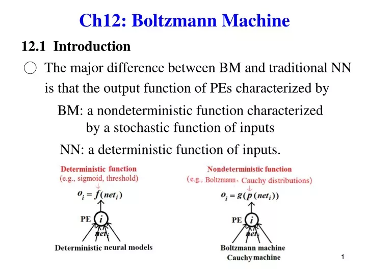
Ch12: Boltzmann Machine. 12.1 Introduction. ○ The major difference between BM and traditional NN is that the output function of PEs characterized by. BM: a nondeterministic function characterized by a stochastic function of inputs.

E N D
Ch12: Boltzmann Machine 12.1 Introduction ○ The major difference between BM and traditional NN is that the output function of PEs characterized by BM: a nondeterministic function characterized by a stochastic function of inputs NN: a deterministic function of inputs. 1
○ Prerequisites for learning BM: 1) information theory, 2) statistical dynamics, 3) simulated annealing, 4)energy function. 12.1.1 Information Theory probability of occurrence If e occurs, receive bits of information. Bit: the amount of information receives when any of two equally probable alternatives is observed, i.e.,
If This means that if we know for sure that an event will occur, its occurrence provides no information at all. 。 Consider a sequence output of symbols from the source with occurring probabilities Zero-memory source: the probability of sending each symbol is independent of symbols previously sent. The amount of information from each received symbol is
Entropyof the information source: the average amount of information received per symbol • The information system, whose symbols occur with equal probability, has the largest degree of unpredicatability (the maximum entropy. Proof:
If is a source with equiprobable symbols, then The second term in (1) is zero where informationgain(Kullback-Leibler divergencebetween and )
12.1.2 Statistical Mechanics – Deals with ensembles, each of which contains a large number of identical small systems, e.g., thermodynamics, quantum mechanics
Example: A thermodynamic system at temperature T is given sufficient time to reach an equilibrium state in which the probability that a particle i has an energy following the Boltzmann (Gibbs) distribution where T : Kelvins temperature : Boltzmann constant 8
: Partition function The system energy at the equilibrium state is in an average sense • The coarsenessof particle i with energy : The entropy of the system is the average coarseness of its constituent particles 9
○ Two systems with the respective entropies Suppose they have the same energy, i.e., Suppose follows Boltzmann distribution, i.e., The entropy difference between two systems
* A system whose constituent small systems with their energy follow the Boltzmann distribution has the largest entropy.
12.1.3 Simulated Annealing Neural networks achieve purposes (i.e., training and production) by minimizing or maximizing some objective functions. Learning process -- e.g., Adaline (CGD), Backpropagation (MSE) Recall process -- e.g., BAM (Energy), Hopfield model (Energy) Methods: gradient descent, hill climbing Difficulties: local extremes Simulated annealing reduces the possibility of falling into a local extreme
Idea: Reduces the possibility of falling into a local extreme by shaking 14
Example: A silicon boule being grown in a furnace First raise temperature, then Mildly cool downRapid cool down solid structure fragile structure lower energy (stable) higher energy (unstable) Simulated annealing starts with a high temperature and gradually lower temperature while processing. High temperature<--> vigorous shaking Low temperature<--> gentle shaking
12.1.4 Energy Function • Dynamic system: a system whose state changes with time. • State: a collection of adaptable quantitative and qualitative items that characterizing the system, e.g., weights, data flows …..
Example: where x,y: input and output vectors; both are bipolar.
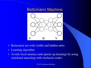
12.2. Boltzmann Machine ○ Three different types of BM: 1. Completion network i) 2 layers: hidden and visible layers, ii) Fully interconnected between layers and among units on each layer iii) All connections are bidirectional 19
2. I/O network • The visible units are divided into input and output units ii) No connections among input units • Connections from input to other units are unidirectional • All other connections are bidirectional.
3. Restricted Network • Consists of two layers: visible layer v, and hidden layer h. (2) There is no connection among the visible or hidden neurons. (3) No temperature parameter employed, i.e., no annealing process involved in both training and production 21
12.2.1 Boltzmann Completion Network Input patterns: binary vectors 。 The systemenergy n : # units (both hidden and visible) : the output of the ith unit
Given an incomplete pattern where u: unknown of a stored pattern To recall x 1. Set the visible units to the known values specified by 2. Set the unknown visible units and the hidden units to random values from {0,1} 3. Set the initial temperature to a large 4. Calculate the net input of a randomly selected unit j ( hidden or visible node)
5. Calculate 6. Repeat 4 and 5 for all units (one processing cycle) 7. Repeat 6 several cycles, until thermal equilibrium ( ) has been reach at T 8. Lower T and repeat steps 4 though 7 Once the network has reached equilibrium at small T, the network has the minimal energy and the result is on the visible layer.
。 The probability that the network is in state x: Define events: Probabilities: P(B) is the marginal probability of C w.r.t. A. 25
Logistic function 26
◎ Boltzmann I/O Network The input vector is clamped at the visible layer and is never updated All hidden and output units are updated according to simulated annealing 12.2.2. Learning ◎ The learning algorithm attempts to build a probability model of the population based on the given examples. There are many different models that are consistent with the examples. How to choose among the various models?
Insist the model to lead to the most homogeneous distributionof input patterns consistent with the examples supplied. 。 Example: 3D vectors (_,_,_) in a population P, whose components Suppose vectors of type (1,_,_) have 40% in P. There are many choices, e.g., The most homogeneous distribution is
◎The learning algorithm discovers a set of weights that minimized the information gain of the observed (clamped) probability distribution w.r.t. the Boltzmann (unclamped) distribution. 。 The information gain of system w.r.t. system defined as indicates the difference between the probability distributions of these two systems.
。 Outline of training the Boltzmann machine 1. Raise the temperature of the BM. 2. Anneal the system until equilibrium is reached at some low temperature. 3. Adjust the weights of the BM so that G is reduced. 4. Repeat 1~3 until the observed probability distribution approximates the Boltzmann distribution. The above procedure uses the techniques of gradient descent (3) on G and simulated annealing (1, 2).
。 Given a set of examples for being learned, define as the set of all possible vectors that may appear on the hidden units Clamp the outputs of visible units to each Let : the probability that the visible units are clamped to . “+” indicates clamped visible units : the joint probability that is clamped to the visible units and appears on the hidden layer.
Let: the probability that appears on the visible layer without clamping visible units. “-” indicates unclamped visible units : the joint probability that appears on the visible layer and appears on the hidden layer without clamping visible units An unclamped (free-running) system in equilibrium at some T, the probability distribution is Boltzmann , where : either a visible or a hidden unit. 32
Information gain: independent of clamping ) 33
i.e., if is on the visible layer, then the probability that will appear on the hidden layer should not depend on whether got the visible layer by being clamped or by free running.
Weight update: : compute the frequency that and are both active averaged over all possible combinations of and 。 Training the Boltzmann machine Initial weights are randomly assigned between 0 and 1. 1. Clamp one training vector to the visible units 2. Anneal the network until equilibrium at the lowest temperature (one cycle) 39
3. Continue for several processing cycles. After each cycle, determine the pairs of connected units which are on simultaneously (i.e. co-occurrence). 4. Average the co-occurrence results (per cycle) 5. Repeat 1~4 for all training vectors Average the co-occurrence results (per training vector) to get an estimate of 6. Unclamped the visible units. Run through 2~5 for calculating 7. Change weights according 8. Repeat 1~7 until is sufficiently small.
12.2.3. Practical Considerations 。 The learning process is very slow. Geman & Geman show that the temperature must be reduced according to : starting temperature where : the nth processing cycle ◎ Cauchy machine a. Based on Cauchy distribution b. Annealing temperature follows
12.3. Symptom-Diagonosis Application – Diagnose why a car will not start 。 Symptoms: 1. Does nothing, 2. Click, 3. Grinds, 4. Cranks, 5. No spark, 6. Cable hot, 7. No gas 。 Possible causes: 1. Battery, 2. Solenoid, 3. Starter, 4. Wires, 5. Distributor, 6. Fuel Pump 。 Relationships
。 Solution: 1. Boltzmann I/O Network 2. 6 training vector pairs e.g., training pair 3 I (0 1 0 0 0 1 0) clicks, cable hot O (0 1 0 0 0 0) solenoid
Restricted Boltzmann Machine • Consists of two layers: visible layer v, and hidden layer h. (2) There is no connection among the visible or hidden neurons. (3) No temperature parameter employed, i.e., no annealing process involved in both training and production 44
Bernoulli-Bernoulli RBM: The energy function for a configuration (v, h): The probability with a configuration (v, h): 45
Gaussian-Bernoulli RBM: The energy function for a configuration (v, h): The probability with a configuration (v, h): 48
The conditonalprobabilitiesp(h | v), p(v | h): • Given v, all hidden nodes are conditional independent (since there is no connections among hidden nodes), i.e., p(h|v) = p(h1|v) … p(hn|v). Likewise, given h, all visible nodes are conditional independent. 49
When input v, passing through p(h|v) we obtain h. Next, passing through p(v|h) we obtain v1. If v1 = v, the h can be a good representation or feature of v. How to train a RBM? Given the energy of a configuration of the RBM, The probability characterized by the configuration is 50