PARTIAL DERIVATIVES

1. 14 PARTIAL DERIVATIVES

2. PARTIAL DERIVATIVES 14.3 Partial Derivatives • In this section, we will learn about: • Various aspects of partial derivatives.

3. INTRODUCTION • On a hot day, extreme humidity makes us think the temperature is higher than it really is. • In very dry air, though, we perceive the temperature to be lower than the thermometer indicates.

4. HEAT INDEX • The National Weather Service (NWS) has devised the heat indexto describe the combined effects of temperature and humidity. • This is also called the temperature-humidity index, or humidex, in some countries.

5. HEAT INDEX • The heat index Iis the perceived air temperature when the actual temperature is T and the relative humidity is H. • So, Iis a function of T and H. • Wecan write I =f(T, H).

6. HEAT INDEX • This table of values of Iis an excerpt from a table compiled by the NWS.

7. HEAT INDEX • Let’s concentrate on the highlighted column. • It corresponds to a relative humidity of H = 70%. • Then, we are considering the heat index as a function of the single variable T for a fixed value of H.

8. HEAT INDEX • Let’s write g(T) = f(T, 70). • Then, g(T) describes: • How the heat index Iincreases as the actual temperature T increases when the relative humidity is 70%.

9. HEAT INDEX • The derivative of g when T = 96°F is the rate of change of Iwith respect to T when T = 96°F:

10. HEAT INDEX • We can approximate g’(96) using the values in the table by taking h = 2 and –2.

11. HEAT INDEX • Averaging those values, we can say that the derivative g’(96) is approximately 3.75 • This means that: • When the actual temperature is 96°F and the relative humidity is 70%, the apparent temperature (heat index) rises by about 3.75°F for every degree that the actual temperature rises!

12. HEAT INDEX • Now, let’s look at the highlighted row. • It corresponds to a fixed temperature of T = 96°F.

13. HEAT INDEX • The numbers in the row are values of the function G(H) = f(96, H). • This describes how the heat index increases as the relative humidity H increases when the actual temperature is T = 96°F.

14. HEAT INDEX • The derivative of this function when H = 70% is the rate of change of I with respect to H when H = 70%:

15. HEAT INDEX • By taking h = 5 and –5, we approximate G’(70) using the tabular values:

16. HEAT INDEX • By averaging those values, we get the estimate G’(70) ≈ 0.9 • This says that: • When the temperature is 96°F and the relative humidity is 70%, the heat index rises about 0.9°F for every percent that the relative humidity rises.

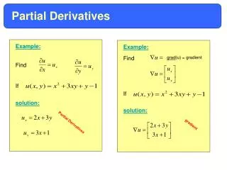
17. PARTIAL DERIVATIVES • In general, if f is a function of two variables x and y, suppose we let only x vary while keeping y fixed, say y = b, where b is a constant. • Then, we are really considering a function of a single variable x: • g(x) = f(x, b)

18. PARTIAL DERIVATIVE • If g has a derivative at a, we call it the partialderivative of f with respect to xat (a, b). • We denote it by: • fx(a, b)

19. PARTIAL DERIVATIVE Equation 1 • Thus, fx(a, b) = g’(a) where g(x) = f(a, b)

20. PARTIAL DERIVATIVE • By the definition of a derivative, we have:

21. PARTIAL DERIVATIVE Equation 2 • So, Equation 1 becomes:

22. PARTIAL DERIVATIVE • Similarly, the partial derivative of f with respect to yat(a, b), denoted by fy(a, b), is obtained by: • Keeping x fixed (x = a) • Finding the ordinary derivative at bof the function G(y) = f(a, y)

23. PARTIAL DERIVATIVE Equation 3 • Thus,

24. PARTIAL DERIVATIVES • With that notation for partial derivatives, we can write the rates of change of the heat index Iwith respect to the actual temperature T and relative humidity H when T = 96°F and H = 70% as: • fT(96, 70) ≈ 3.75 fH(96, 70) ≈ 0.9

25. PARTIAL DERIVATIVES • If we now let the point (a, b) vary in Equations 2 and 3, fx and fy become functions of two variables.

26. PARTIAL DERIVATIVES Equations 4 • If f is a function of two variables, its partial derivativesare the functions fx and fy defined by:

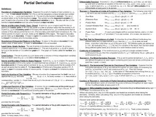
27. NOTATIONS • There are many alternative notations for partial derivatives. • For instance, instead of fx, we can write f1 or D1f (to indicate differentiation with respect to the firstvariable) or ∂f/∂x. • However, here, ∂f/∂x can’t be interpreted as a ratio of differentials.

28. NOTATIONS FOR PARTIAL DERIVATIVES • If z = f(x, y), we write:

29. PARTIAL DERIVATIVES • To compute partial derivatives, all we have to do is: • Remember from Equation 1 that the partial derivative with respect to x is just the ordinaryderivative of the function g of a single variable that we get by keeping y fixed.

30. RULE TO FIND PARTIAL DERIVATIVES OF z = f(x, y) • Thus, we have this rule. • To find fx, regard y as a constant and differentiate f(x, y) with respect to x. • To find fy, regard x as a constant and differentiate f(x, y) with respect to y.

31. PARTIAL DERIVATIVES Example 1 • If f(x, y) = x3 + x2y3 – 2y2find fx(2, 1) and fy(2, 1)

32. PARTIAL DERIVATIVES Example 1 • Holding y constant and differentiating with respect to x, we get: fx(x, y) = 3x2 + 2xy3 • Thus, fx(2, 1) = 3 . 22 + 2 . 2 . 13 = 16

33. PARTIAL DERIVATIVES Example 1 • Holding x constant and differentiating with respect to y, we get: fy(x, y) = 3x2y2 – 4y • Thus, fy(2, 1) = 3 . 22 . 12 – 4 . 1 = 8

34. GEOMETRIC INTERPRETATION • To give a geometric interpretation of partial derivatives, we recall that the equation z = f(x, y) represents a surface S (the graph of f). • If f(a, b) = c, then the point P(a, b, c) lies on S.

35. GEOMETRIC INTERPRETATION • By fixing y = b, we are restricting our attention to the curve C1 in which the vertical plane y = b intersects S. • That is, C1 is the trace of Sin the plane y = b.

36. GEOMETRIC INTERPRETATION • Likewise, the vertical plane x = a intersects S in a curve C2. • Both the curves C1 and C2 pass through P.

37. GEOMETRIC INTERPRETATION • Notice that the curve C1 is the graph of the function g(x) = f(x, b). • So, the slope of its tangent T1at P is: g’(a) = fx(a, b)

38. GEOMETRIC INTERPRETATION • The curve C2 is the graph of the functionG(y) = f(a, y). • So, the slope of its tangent T2at P is: G’(b) = fy(a, b)

39. GEOMETRIC INTERPRETATION • Thus, the partial derivatives fx(a, b) and fy(a, b) can be interpreted geometrically as: • The slopes of the tangent lines at P(a, b, c) to the traces C1and C2 of S in the planes y = b and x = a.

40. INTERPRETATION AS RATE OF CHANGE • As seen in the case of the heat index function, partial derivatives can also be interpreted as rates of change. • If z = f(x, y), then ∂z/∂x represents the rate of change of z with respect to x when y is fixed. • Similarly, ∂z/∂y represents the rate of change of zwith respect to y when x is fixed.

41. GEOMETRIC INTERPRETATION Example 2 • If • f(x, y) = 4 – x2 – 2y2 • find fx(1, 1) and fy(1, 1) and interpret these numbers as slopes.

42. GEOMETRIC INTERPRETATION Example 2 • We have: • fx(x, y) = -2xfy(x, y) = -4y • fx(1, 1) = -2 fy(1, 1) = -4

43. GEOMETRIC INTERPRETATION Example 2 • The graph of f is the paraboloid z = 4 – x2 – 2y2 • The vertical plane y = 1 intersects it in the parabola z = 2 – x2, y = 1. • As discussed, we label it C1.

44. GEOMETRIC INTERPRETATION Example 2 • The slope of the tangent line to this parabola at the point (1, 1, 1) is: fx(1, 1) = -2

45. GEOMETRIC INTERPRETATION Example 2 • Similarly, the curve C2 in which the plane x = 1 intersects the paraboloid is the parabola z = 3 – 2y2, x = 1. • The slope of the tangent line at (1, 1, 1) is: fy(1, 1) = – 4

46. GEOMETRIC INTERPRETATION • This is a computer-drawn counterpart to the first figure in Example 2. • The first part shows the plane y = 1 intersecting the surface to form the curve C1. • The second part shows C1 and T1.

47. GEOMETRIC INTERPRETATION • We have used the vector equations: • r(t) = <t, 1, 2 – t2> for C1 • r(t) = <1 + t, 1, 1 – 2t> for T1

48. GEOMETRIC INTERPRETATION • Similarly, this figure corresponds to the second figure in Example 2.

49. PARTIAL DERIVATIVES Example 3 • If • calculate

50. PARTIAL DERIVATIVES Example 3 • Using the Chain Rule for functions of one variable, we have: