Download
1 / 86
880 likes | 1.05k Views
Light Pollution Stellar Evolution. Lab Notes. Be sure you have started your “ report ” lab. Constellation presentations next week. Observatory field trips…. Night Lights. http://apod.nasa.gov/apod/ap101104.html. Limiting Magnitude and Light Pollution. Limiting Magnitude.

E N D
Light Pollution Stellar Evolution 2
Lab Notes • Be sure you have started your “report” lab. • Constellation presentations next week. • Observatory field trips… 3
Night Lights • http://apod.nasa.gov/apod/ap101104.html 4
Limiting Magnitude and Light Pollution 5
Limiting Magnitude • Limiting Magnitude is a measure of the dimmest star visible from a given location. • Center of a big city: ~2.0 • Suburbs: ~4.5 • Downtown Durango: ~5.5 • La Plata County (FLC observatory): ~6.5 • Depends on observer experience • Depends on local glare • Depend on how dark adapted your eyes are. You should wait 20-30 minutes to measure this. 6
Limiting Magnitude • Use stars of known magnitude (e.g. Little Dipper) 7
Limiting Magnitude • Count the stars in a well-defined region • Chose one of the predefined star regions that is overhead • Count the number of stars visible within the region boundary • Look up the number on the published tables to find the corresponding limiting magnitude 8
Limiting Magnitude Alpha-Epsilon-Beta Gem stars LM 1 1.2 2 2.4 3 3.2 4 3.9 5 4.3 6 5.0 7 5.1 8 5.3 9 5.6 10 5.7 11 5.9 12 6.1 13 6.2 14 6.3 15 6.4 16 6.5 18 6.6 20 6.7 22 6.9 23 7.0 25 7.2 30 7.5 10
How many Stars Can You See? Magnitude Range Cumulative Stars % Increase Seen -1-1.50 to -0.51 2 - 0-0.50 to +0.49 8 400% 1+0.50 to +1.49 22 275% 2 +1.50 to +2.49 93 423% 3 +2.50 to +3.49 283 304% 4 +3.50 to +4.49 893 316% 5 +4.50 to +5.49 2,822 316% 6 +5.50 to +6.49 8,768 311% 7 +6.50 to +7.49 26,533 303% 8 +7.50 to +8.49 77,627 293% 9 +8.50 to +9.49 217,689 280% 10 +9.50 to +10.49 626,883 288% 11 +10.50 to +11.49 1,823,573 291% 12 +11.50 to +12.49 5,304,685 291% 13 +12.50 to +13.49 15,431,076 291% 14 +13.50 to +14.49 44,888,260 291% 15 +14.50 to +15.49 130,577,797 291% 16 +15.50 to +16.49 379,844,556 291% 17 +16.50 to +17.49 1,104,949,615 291% 18 +17.50 to +18.49 3,214,245,496 291% 19 +18.50 to +19.49 9,350,086,162 291% 20 +19.50 to +20.49 27,198,952,706 291% 11
How many Stars Can You See? • Dark-adapted naked eye (1x7 binoculars) • Can see to magnitude 6.5 -> ~104 stars • Light gathering ability scales with area. • Magnitude Increase = log10(Area increase) / 0.4 • 10x50 binoculars ~50x area -> +4.25 magnitudes • 16” SCT ~64x area -> +4.5 magnitudes • 10m Keck telescope ~625x area -> +7 magnitudes 12
How many Stars Can You See? • So for naked eye observing • 10x50 binoculars • 50x area • +4.25 magnitudes (to 10.75) > 106 stars • 16” SCT • 64x area • +4.5 magnitudes (to 15.25) > 108 stars • 10m Keck telescope • 625x area • +7 magnitudes (to 22.75) > 1011 stars 13
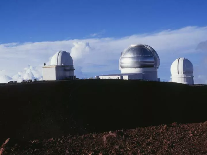
Light Pollution • Generally not an issue in La Plata county. • Durango has a dark sky ordinance, but only for new construction. • Fort Lewis is making progress with outside light fixtures. 15
Light Pollution Earth at Night Credit: C. Mayhew & R. Simmon (NASA/GSFC), NOAA/ NGDC, DMSP Digital Archive 16
Light Pollution From IDA Website: http://www.darksky.org/images/sat.html 17
Light Pollution You Are Here Observatory 18
Figure 10.15Hipparcos H–R Diagram • Plot the luminosity vs. temperature. • This is called a Hertzsprung-Russell (H-R) diagram 19
What fraction of the stars on an H-R diagram are on the main sequence • 0-50% • 50-70% • 70-80% • >80% 20
What fraction of the stars on an H-R diagram are on the main sequence • 0-50% • 50-70% • 70-80% • >80% 21
Distance Scale • If you know brightness and distance, you can determine luminosity. • Turn the problem around… 22
Distance Scale • If you know brightness and distance, you can determine luminosity. • Turn the problem around… • If a star is on the main sequence, then we know its luminosity. So • If you know brightness and luminosity, you can determine a star’s distance. 23
Distance Scale • Spectroscopic Parallax - the process of using stellar spectra to determine distances. • Can use this distance scale out to several thousand parsecs. 24
Figure 11.16Atomic Motions • Low density clouds are too sparse for gravity. • A perturbation could cause one region to start condensing. 27
http://discovermagazine.com/2009/interactive/star-formation-game/http://discovermagazine.com/2009/interactive/star-formation-game/ • google “star formation game” 30
H-R diagram review • The H-R diagram shows luminosity vs. temperature. • It is also useful for describing how stars change during their lifetime even though “time” is not on either axis. • How to do this may not be obvious. • Exercise - Get in groups of ~four and get out a blank piece of paper. 31
Group Exercise • As a group, create a diagram with “financial income” on the vertical axis, and “weight” on the horizontal axis. • Use this graph to describe the past and future of a fictitious person (or a group member). • Label significant events, for example • birth • college • retirement • death 32
Stellar Evolution 1 - interstellar cloud - vast (10s of parsecs) 2(and 3) - a cloud fragment may contain 1-2 solar masses and has contracted to about the size of the solar system 4 - a protostar • center ~1,000,000 K • Too cool for fusion, but hot enough to see. (photosphere ~3000 K) • radius ~100x Solar 33
How would the luminosity of a one-solar-mass protostar compare to the sun? A) Less than .1x as bright B) A little lower. C) About the same. D) A little brighter E) More than 10x brighter 34
How would the luminosity of a one-solar-mass protostar compare to the sun? A) Less than .1x as bright B) A little lower. C) About the same. D) A little brighter E) More than 10x brighter 35
Figure 11.21Newborn Star on the H–R Diagram 5 - Gravity still dominates the radiation pressure, so the star continues to shrink. 37
Stars A and B formed at the same time. Star B has 3 times the mass of star A. Star A has an expected lifetime of 3 billion years. What is the expected lifetime of star B? A) more than 9 billion years B) about 9 billion years C) 3 billion years D) about 1 billion years E) less than 1 billion years 41
Stars A and B formed at the same time. Star B has 3 times the mass of star A. Star A has an expected lifetime of 3 billion years. What is the expected lifetime of star B? A) more than 9 billion years B) about 9 billion years C) 3 billion years D) about 1 billion years E) less than 1 billion years 42
Stellar Lifetimes • Proportional to mass • Inversely proportional to luminosity • Big stars are MUCH more luminous, so they use their fuel MUCH faster. • The distribution of star types is representative of how long stars spend during that portion of their life. • Example - snapshots of people. 43
Figure 11.21Newborn Star on the H–R Diagram 5 - Gravity still dominates the radiation pressure, so the star continues to shrink. 49
Figure 11.21Newborn Star on the H–R Diagram 5 - Gravity still dominates the radiation pressure, so the star continues to shrink. Can have violent “winds” streaming outwards; often bipolar flow from poles; T-Tauri phase 50