Download
1 / 56
560 likes | 703 Views
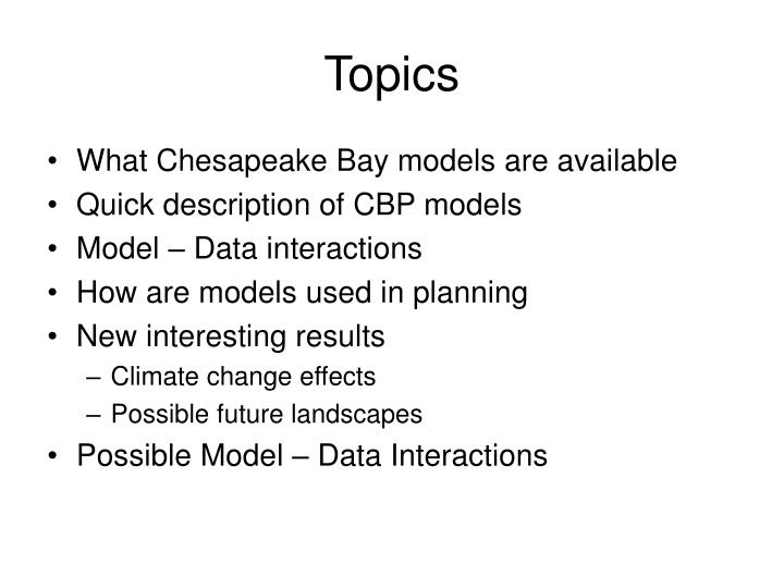
Topics. What Chesapeake Bay models are available Quick description of CBP models Model – Data interactions How are models used in planning New interesting results Climate change effects Possible future landscapes Possible Model – Data Interactions. Environmental Models. Uses

E N D
Topics • What Chesapeake Bay models are available • Quick description of CBP models • Model – Data interactions • How are models used in planning • New interesting results • Climate change effects • Possible future landscapes • Possible Model – Data Interactions
Environmental Models • Uses • Fill in gaps in data – Hindcast (calibration) • Spatial • Temporal • Functional • Prediction – Forecast – Scenario • Answer what-if? questions
http://ccmp.chesapeake.org/CCMP/models.php • Chesapeake-related open source modeling effort gaining some momentum • Several versions of Bay models available • More watershed models in development
Place of Models in Chesapeake Bay Program Decision Structure Managers Modeling Research Analysis Monitoring Ecosystem
Decision Support System Land Use Change Model Criteria Assessment Procedures Bay Model Watershed Model COAST Data Airshed Model Effects Allocations
Hourly Values: Rainfall Snowfall Temperature Evapotranspiration Wind Solar Radiation Dewpoint Cloud Cover Annual or Monthly: Land Use Acreage Conservation Practices Fertilizer Manure Atmospheric Deposition Point Sources Septic Loads Quick overview of watershed model Calibration HSPF Daily output compared To observations
Hourly Values: Rainfall Snowfall Temperature Evapotranspiration Wind Solar Radiation Dewpoint Cloud Cover Snapshot: Land Use Acreage Conservation Practices Fertilizer Manure Atmospheric Deposition Point Sources Septic Loads Quick Overview of Watershed Model Scenarios Hourly output is summed over 10 years of hydrology to compare against other management scenarios HSPF “Average Annual Flow-Adjusted Loads”
High Density Pervious Urban High Density Impervious Urban Low Density Pervious Urban Low Density Impervious Urban Construction Extractive Forest Disturbed Forest Natural Grass Composite Crop with Manure (high till) Composite Crop with Manure (low till) Composite Crop without Manure Alfalfa Nursery Pasture Degraded Stream bank Animal Feeding Operations Hay with Nutrients Hay without Nutrients Each segment consists of separately-modeled land uses
Automated Calibration • Ensures even treatment across jurisdictions • Fully documented calibration strategy • Repeatable • Makes Calibration Feasible • Enables uncertainty analysis
RiverReach How do we calibrate? Reasonable values of sediment, nitrogen, and phosphorus Observations of flow, sediment, nitrogen, and phosphorus
Calibration of hydrology • Model Structure • Files External Transfer Module 3 Optimization Routine
Calibration of land nutrients and sediment Optimization Routine Compare to literature values
Calibration of River Water Quality • Process • Parameter • Files • Model Structure • Files Optimization Routine
Hourly Values: Rainfall Snowfall Temperature Evapotranspiration Wind Solar Radiation Dewpoint Cloud Cover Snapshot: Land Use Acreage Conservation Practices Fertilizer Manure Atmospheric Deposition Point Sources Septic Loads Use of the Watershed model in Decision Making Hourly output is summed over 10 years of hydrology to compare against other management scenarios HSPF “Average Annual Flow-Adjusted Loads”
From the Chesapeake Bay Commission Report: Cost-Effective Strategies for the Bay December, 2004
Nitrogen Load Indicator Watershed model indicator of source sector for nitrogen loads to the Bay
Chesapeake Bay and Tidal Tributary Nutrient and/or Sediment Impaired Waterbodies AllocationsExample Note: Representation of 303(d) listed waters for nutrient and/or sediment water quality impairments for illustrative purposes only. For exact 303(d) listings contact EPA (http://www.epa.gov/owow/tmdl/). Impaired Water Unimpaired Water Section 1: What Do We Want to Achieve
Decision Support System Land Use Change Model Criteria Assessment Procedures Bay Model Watershed Model COAST Data Airshed Model Effects Allocations
Judging Progress Tier2 Tier1 Tier3
The Great Divide Tier3 Drastic Option
Effect of Geographic Targeting Tier3 Drastic Option
Effect of Geographic Targeting Tier3 Efficient Option Drastic Option
Allocating Maximum Loads for Nutrient and Sediment Pollution Susquehanna Upper Western Shore Potomac Pax Upper Eastern Shore Rapp York James VA Eastern Shore
Allocating Maximum Loads for Nutrient and Sediment Pollution New York Pennsylvania Maryland District of Columbia West Virginia Delaware Virginia
Allocating Maximum Loads for Nutrient and Sediment Pollution Then running many scenarios to determine a reasonable plan for each area meet their nutrient goals
Estimated Climate Change Effects in the Chesapeake Region In our region, temperatures are estimated to increase with a high degree of certainty, and precipitation to increase especially at higher rainfall events with a moderate degree of certainty. How this effects flow in the watershed hangs in a hydrologic balance between precipitation and evapotranspiration. About half the annual Chesapeake watershed precipitation inputs are lost by evapotranspiration.
Mean Annual Temperature Observed Temperature and Precipitation Trends (1901-1998) Looking back over the observed record for the last century. Annual Precipitation Total Red = increase Blue = decrease Green = increase Brown = decrease
Observed trends in precipitation by size class (percent per century, 1910-1996) National Average Source: Karl and Knight, 1998
Global Climate Models (GCMs) Used Seven Global Climate Models were used from the CARA analysis. These GCMs “differ in their output for a number of reasons, including spatial resolution in the atmosphere and ocean, treatments of land hydrology, and treatments of sea ice.” They are: • CCCM – Canadian Centre for Climate Modeling and Analysis • CSIRO - Australia’s Commonwealth Scientific and Industrial • Research Organization • ECHM - German High Performance Computing Centre for Climate • and Earth System Research • GFDL - Geophysical Fluid Dynamics Laboratory • HDCM - Hadley Centre for Climate Prediction and Research • NCAR - National Center for Atmospheric Research • CCSR - Univ. of Tokyo, Center for Climate System Research/ • National Institute for Environmental Studies
Two emission scenarios from the UN’s Intergovernmental Panel on Climate Change (IPCC) were used. • A2 emission scenario - A very heterogeneous world of economic growth where the underlying theme is self-reliance and preservation of local identities. Fertility patterns across regions converge slowly, which results in continuously increasing population. Economic development is primarily regionally oriented and per capita economic growth and technological change are more fragmented and slower than other storylines. • B2 emission scenario - A world in which the emphasis is on local solutions to economic, social, and environmental sustainability. It is a world with continuously increasing global population, but at a lower rate than A2, and with intermediate levels of economic development, and technological change. While the scenario is oriented toward environmental protection and social equality, it focuses on local and regional levels. Projected CO2 concentrationsusing IPCC “SRES” storylines
flash upper 10 flash upper 30 uniform multiplier Rationale for Different Methods of Modifying Precipitation
Climate Scenarios } • 7 models • 2 futures • = 14 scenarios for each precip method • 3 precipitation methods • Chose high, medium, and low effect for each precip method • 9 bay-wide scenarios
CBP Management Under A Changing Climate • Planning for long-term Bay restoration may involve the consideration of new questions: • What are the potential impacts of climate change on water quality and living resources? • How will our tributary strategies and other management actions perform under changing climatic conditions? • What are the implications for water resources, such as water supply and flood control measures.
Model data interactions • Direct calibration • Models identify monitoring priorities spatially, temporally, and functionally • Data analyses and empirical models (estimator, sparrow) can give a separate estimate of hindcast Data priorities calibration priorities calibration e models M models comparisons
Empirical vs mechanistic • Empirical • Known accuracy • Limited to spatial/temporal range and scale of the data • Mechanistic • Can predict beyond the data • Unknown accuracy generally
2002 Chesapeake Bay Sediment SPARROW Load = B0 * {sources} * B1 * {loss mechanisms}