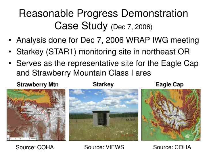
Reasonable Progress Demonstration Case Study (Dec 7, 2006)

1. Reasonable Progress DemonstrationCase Study (Dec 7, 2006) • Analysis done for Dec 7, 2006 WRAP IWG meeting • Starkey (STAR1) monitoring site in northeast OR • Serves as the representative site for the Eagle Cap and Strawberry Mountain Class I ares Starkey Eagle Cap Strawberry Mtn Source: VIEWS Source: COHA Source: COHA

2. Proposed Format for DemonstratingReasonable Progress

3. Regional Haze Rule • Promulgated in 1999 • Requires states to set RPGs based on 4 statutory factors and consideration of a URP • URP = 20% reduction in manmade haze (dv) per planning period (10 years) • URP heavily dependent on: • Assumptions regarding future natural conditions • Contribution of non-WRAP sources to baseline • Representativeness of 2000-04 baseline • 24 of the 77 Class I sites have no more than 3 years of data in baseline period • These issues more accute in the West

4. Why A Species-Based Approach? • Isolate some of the URP issues previously noted • Species differ significantly from one another in their: • Contribution to visibility impairment • Spatial and seasonal distributions • Source types • Contribution from natrual and international sources • Emissions data quality • Atmospheric science quality • Tools available for assessment and projection

6. What Is A Potential Process? • For each site and species … • Estimate progress expected from Base Case + BART in 2018 • Determine any other LTSs which may be reasonable for that pollutant and recalculate 2018 species concentration • Add up improvements from all species into dv • This becomes the RPG for the 20% worst days • Explain why this is less than URP • Large international and natural contributions, large uncertainties in dust inventory preclude action, etc.

7. Determine URP for a species Is Base+BART projection better than URP? Is WRAP Anthro reduction > 20%? N N Evaluate emission & air quality trends more closely Y Y Interstate coop key. Identify LTSs for these sources considering the 4 RPG and other factors identified in the RHR. Are there any important uncontrolled or undercontrolled sources? Are there any important uncontrolled sources? Y Y Adopt, commit to adopt, or commit to further evaluation. N* N Determine reductions at C1A. Repeat for other species. Add up all species reductions to get a RPG for worst days. Eplain why it’s less than default URP but still reasonable. Set goal for best days. * Note, if no LTS beyond BART is developed, then the 4 RPG factors are inherently taken into account via BART.

8. Determining Non-BART LTSs • Determine species glidepath and 2018 URP value • Estimate progress expected from Base Case + BART in 2018 • If progress is better than or equal to 2018 URP: • Check inventory for “important sources” which may be uncontrolled • If progress is worse than 2018 URP, but WRAP antho contribution declines by at least 20%: • Check inventory for important sources which may be uncontrolled

9. Determining Non-BART LTSs • If progress is worse than 2018 URP, and WRAP antho contribution declines by less than 20%: • Evaluate air quality & emission trends in more detail • Check inventory for important sources which may be uncontrolled or undercontrolled • Identify LTSs for these sources considering the 4 RPG factors and 7 LTS factors, where applicable • Either adopt these strategies, commit to adopting them post 2007, or commit to evaluating them further

10. “Important Sources” • Identified and qualitatively ranked based on some or all of the following: • Size, proximity, current/potential degree of control, feasibility of control, cost effectiveness, etc. • If point sources important, identify ~10 facilities • If area sources important, identify 3-5 categories • Identification of important sources should not be limitted by state boundaries

11. Case Study

12. Eagle Cap / Strawberry MountainBaseline Extinction Budget Source: WRAP Technical Support System >> Resources >> Monitoring >> Composition

13. Eagle Cap / Strawberry MountainSpecies Trends and URP Glidepaths Source: WRAP Technical Support System >> Resources >> Monitoring >> Time Series

14. Upwind Residence TimeOn 20% Wost Visibility Days (2000-04) Source: WRAP Technical Support System >> Resources >> Area of Interest >> Weighted Emission Potential

15. Ammonium Nitrate (NO3)

16. NO3 • Is the Base+BART projection better than URP? • Yes: CMAQ base case projections for 2018 show a 25% reduction in extinction due to NO3. • Results do not yet include BART • Results not yet available on TSS • Precise projection method not yet finalized • WRAP anthro reduction is 33% • See PSAT results on next slide

17. NO3 • Are there any important uncontrolled upwind sources? • Use TSS to examine inventory upwind • PSAT results • PMF results • WEP results • Emission inventories

18. NO3 PSAT Results2002 and 2018 base cases Source: WRAP Technical Support System >> Resources >> Area of Interest >> SOx/NOx Tracer

19. Source: Chart made after manipulation of data posted on WRAP Causes of Hase Website: http://coha.dri.edu/web/general/tools_PMFModeling.html

20. NO3 WEP Results (2000-04) Source: WRAP Technical Support System >> Resources >> Area of Interest >> Weighted Emission Potenital

21. NO3 WEP Results (2018) Source: WRAP Technical Support System >> Resources >> Area of Interest >> Weighted Emission Potenital

22. Source: WRAP Technical Support System >> Resources >> Emissions

23. Most Likely NOx Sources Significantly Contributing to NO3 at STAR On the 20% Worst Visibility Days * See following slides.

24. NOx Sources > 500 tpy in the 2018 Oregon Point Source Pivot Table Source: WRAP website: Emissions Forum pivot tables: http://www.wrapair.org/forums/ssjf/pivot.html

25. 1996 Point Source NOx Emissions* Illustration Only * Emission maps not yet available on TSS. Hence, the above map is used as a placeholder and is for illustration purposes only. This map was obtained from the Causes of Haze website.

26. 2002 Idaho Area Source NOx Emissions Source: WRAP website: Emissions Forum pivot tables: http://www.wrapair.org/forums/ssjf/pivot.html

27. 2018 Idaho Area Source NOx Emissions Source: WRAP website: Emissions Forum pivot tables: http://www.wrapair.org/forums/ssjf/pivot.html

28. Ammonium Sulfate (SO4)

29. SO4 • Is the Base+BART projection better than URP? • No: CMAQ base case projections for 2018 show only a 1% reduction in extinction due to SO4. • Sources outside the WRAP have a large influence • Results not yet available on TSS • Is WRAP anthro reduction > 20%? • No: PSAT apportionment shows only a 10% reduction from WRAP anthro SO2 sources • BART not yet included, but may likely increase reduction to 20% • Major reductions at Centralia “missed” by selection of 2002 as the base year

30. SO4 • Are there any important uncontrolled upwind sources? • Use TSS to examine inventory upwind • PSAT results • PMF results • WEP results • Emission inventories

31. SO4 PSAT Results 2002 and 2018 base cases Source: WRAP Technical Support System >> Resources >> Area of Interest >> SOx/NOx Tracer

32. Source: Chart made after manipulation of data posted on WRAP Causes of Hase Website: http://coha.dri.edu/web/general/tools_PMFModeling.html

33. SO4 WEP Results (2000-04) Source: WRAP Technical Support System >> Resources >> Area of Interest >> Weighted Emission Potenital

34. SO4 WEP Results (2018) Source: WRAP Technical Support System >> Resources >> Area of Interest >> Weighted Emission Potenital

35. Source: WRAP Technical Support System >> Resources >> Emissions

36. Most Likely SO2 Sources Significantly Contributing to SO4 at STAR On the 20% Worst Visibility Days * See following slides.

37. SO2 Sources > 500 tpy in the 2018 Washington Point Source Pivot Table

38. Significant progress made in WA point sources not reflected in choice of base case years (2002 and 2018). Source: EPA Clean Air Markets Division Website

39. SO2 Sources > 500 tpy in the 2018 Oregon Point Source Pivot Table Note: All these sources are BART-eligible. Source: WRAP website: Emissions Forum pivot tables: http://www.wrapair.org/forums/ssjf/pivot.html

40. 1996 Point Source SO2 Emissions* Illustration Only * Emission maps not yet available on TSS. Hence, the above map is used as a placeholder and is for illustration purposes only. This map was obtained from the Causes of Haze website.

41. 2002 and 2018 Oregon Area Source SO2 Emissions Source: WRAP website: Emissions Forum pivot tables: http://www.wrapair.org/forums/ssjf/pivot.html

42. Organic Carbon (OC)

43. Fraction of Carbon That Is Modern or Fossil Source: National Park Service presentation

44. OC • Is the Base+BART projection better than URP? • No: CMAQ base case projections for 2018 show a 6% reduction in extinction due to OC. • Is WRAP anthro reduction > 20%? • Unclear: Reduction in primary anthro carbon is about 20%, but secondary carbon is a larger contributor and it is unclear what portion is anthro. • These reductions assume implementation of smoke emission reduction techniques (ERTs)

45. OC • Are there any important uncontrolled upwind sources? • Use TSS to examine inventory upwind • CMAQ results • PMF results • WEP results • Emission inventories

46. OC CMAQ Results 2002 and 2018 base cases AORGA Change = +2% AORGB Change = -4% AORGPA Change = -18% Source: WRAP Technical Support System

47. Source: Chart made after manipulation of data posted on WRAP Causes of Hase Website: http://coha.dri.edu/web/general/tools_PMFModeling.html

48. OC WEP Results (2000-04) Source: WRAP Technical Support System >> Resources >> Area of Interest >> Weighted Emission Potenital

49. OC WEP Results (2018) Source: WRAP Technical Support System >> Resources >> Area of Interest >> Weighted Emission Potenital

50. Source: WRAP Technical Support System >> Resources >> Emissions