Download
1 / 20
230 likes | 418 Views
Exploring the Atmosphere: Observational Instruments and Techniques Advanced Study Program (ASP) Summer Colloquium. Boundary Layer Lecture Surface-based: Flux Measurements Andrey A. Grachev 1, 2 (also Christopher W. Fairall 2 and Jeffrey E. Hare 1, 2 )

E N D
Exploring the Atmosphere: Observational Instruments and Techniques Advanced Study Program (ASP) Summer Colloquium Boundary Layer Lecture Surface-based: Flux Measurements Andrey A. Grachev 1, 2 (also Christopher W. Fairall 2and Jeffrey E. Hare 1, 2) 1 Cooperative Institute for Research in Environmental Sciences, University of Colorado, Boulder, Colorado, USA 2 NOAA Earth System Research Laboratory, Boulder, Colorado, USA
Atmospheric Surface Layer (ASL) (constant-flux layer) The atmospheric surface layer (or “constant-flux layer”) occupies the lower 10% of the atmospheric boundary layer, or 50-150 m elevation. This is the region we live in, and some of its characteristics are important for a variety of applications. Strong gradients in wind speed, temperature & other scalars in surface boundary layer exist in ASL. Monin-Obukhovsimilarity scaling is applied in ASL. This theory links mean fields and turbulent fluxes in the surface layer. Eddy flux measurements made in surface layer.
Turbulent Fluxes (definition) Momentum flux (or surface stress): Sensible heat flux: Latent heat flux (moisture flux): Transfer of trace gases (CO2, O3 etc.): where cp is the heat capacity of air at constant pressure, Le is the latent heat of evaporation of water, and rc mixing ratio relative to dry air component.
Monin–Obukhov similarity theory (Obukhov, 1946; Monin and Obukhov, 1954) Monin – Obukhov stability parameter (Monin & Obukhov, 1954): Obukhov length (Obukhov, 1946): Non-dimensional velocity and temperature gradients : Neutral case: Very stable stratification: Free convection: Businger–Dyer (Kansas-type) profiles: for (Flux-gradient relationships) for
Limitations of the Monin–Obukhov similarity theory Upward Momentum Transfer in the Marine Boundary Layer Weak wind at sea is frequently accompanied by the presence of fast travelingocean swell, which dramatically affects momentum transfer. It is found that the mean momentum flux (uw-covariance) decreases monotonically with decreasing wind speed, and reaches zero around a wind speed U 1.5–2 m/s Further decrease of the wind speed (i.e., increase of the wave age) leads to a sign reversal of the momentum flux, implying negative drag coefficient. Upward momentum transfer is associated with fast-traveling swell running in the same direction as the wind, and this regime can be treated as swell regime. The common practice of using the friction velocity as a scaling parameter evidently is invalid for swell conditions since x reaches zero and changes sign. Thus, the standard Monin–Obukhov similarity theory presumably is not applicable to describe the momentum transfer in swell conditions.
Limitations of the Monin–Obukhov similarity theory Ekman Surface Layer Evolving Ekman-type spirals during the polar day observed during JD 507 (22 May, 1998) for five hours from 12.00 to 16.00 UTC (4:00–8:00 a.m. local time, see the legend) observed during SHEBA program. Markers indicate ends of wind vectors at levels 1 to 5 (1.9, 2.7, 4.7, 8.6, and 17.7 m). 3D view of the Ekman spiral for 14:00 UTC JD 507 (local time 6 a.m.), 22 May 1998 (SHEBA data).
Turbulent Flux Measurements Sonic anemometer/thermometer t1 = L / (c + v) ; t2 = L / (c - v); v = 0.5 L (1/t1 – 1/t2); c = 0.5 L (1/t1 + 1/t2); Ts = c2 / 403; T = Ts / (1 + 0.32 e / p) L = path length, t = time of flight c = speed of sound, v = wind velocity T = temperature, Ts = “virtual” temp p = pressure, e = water vapor pressure
Turbulent Flux Measurements Gas Analyser (H2O and CO2 fluxes) Absorptance of a particular gas α = 1 – A / Ao A = power received at absorbing wavelength Ao = power received at non-absorbing wavelength ρ = Pef(α / Pe) [mol m-3] number density ρ = Pef([1 – z A / Ao ] S / Pe) , where Pe is equivalent pressure, S is ‘span’ Channels available for water vapor and carbon dioxide
Turbulent Flux Measurements Eddy Correlation (or Covariance) Method Eddy fluxes calculated as covariances in the time domain, <w’u’>, <w’T’>, <w’c’> etc. Spectra and cospectra in the frequency domain. Frequency sampling rate ~ 10-20 Hz. Averaging period must be long enough to capture low-frequency contributions to eddy fluxes. Averaging periods of 30 min or 1 hr are commonly used. Typical (a) stress cospectra (1998 JD 45.4167), and cospectra of the sonic temperature flux (1997 JD 324.5833) for weakly and moderate stable conditionsmeasured during SHEBA. Typical raw cospectra of the H2O (upper panel) and CO2 (bottom panel) fluxes measured August 31, 2007 at Eureka site, Canada.
Turbulent Flux Measurements Inertial-Dissipation Method Frequency spectra in the inertial subrange (Kolmogorov, 1941):
Turbulent Flux Measurements Bulk Relationships Momentum flux (or surface stress): Sensible heat flux: Latent heat flux (moisture flux): Traditionally, the transfer coefficients are adjusted to neutral conditions using Monin-Obukhov similarity theory. The neutral counterparts of the drag coefficient, Stanton number, and Dalton number are derived from the following relationships: The neutral transfer coefficients uniquely define the aerodynamic roughness length and scalar roughness lengths for temperature and humidity:
Bulk Relationships COARE Flux Algorithm COARE Model History: 1996 - Bulk Meteorological fluxes (Fairall et al., 1996); 2000 – Carbon Dioxide (Fairall et al., 2000); 2003 – Update, version 3.0, 8000 1-hr eddy covariance observations (Fairall et al., 2003); 2004 – DMS and 2006 - Ozone. Air-Sea transfer coefficients as a function of wind speed: latent heat flux (upper panel) and momentum flux (lower panel). The red line is the COARE algorithm version 3.0; the circles are the average of direct flux measurements from 12 ETL cruises (1990-1999); the dashed line the original NCEP model.
Air-Sea Flux Measurements NOAA R/V Ronald H. Brown Using advanced techniques for direct measurement of air-sea fluxes, we have obtained data from oceans around the world. This data has been used to develop parameterizations to estimate air-sea fluxes from mean state variables (wind speed, air temperature, sea temperature, humidity, etc). Air-sea fluxes of heat (latent/sensible) are also fundamental to cloud development (hence, surface energy budget, precipitation, etc).
NOAA R/V Ronald H. Brown Flow distortion study
NOAA R/V Ronald H. Brown NOAA/ESRL Turbulent Flux System
Texas Air Quality Study (TexAQS) R/V Ronald H. Brown cruise track NOAA R/V Ronald H. Brown cruise track during TexAQS-06. The ship departed Charleston, South Carolina on 27 July 2006, arriving initially in Galveston, Texas on 2 August 2006. The cruise track included passages into Port Arthur/Beaumont, Matagorda Bay, Freeport Harbor, Galveston Bay to Barbour’s cut (15 transits), and the Houston Ship Channel (4 transits). The cruise ended in Galveston, Texas on 11 September 2006.
Texas Air Quality Study (TexAQS) R/V Ronald H. Brown, Time Series – Leg 2 Time series of (a) the location code, (b) the air and water temperature, (c) the wind speed and the true wind direction, and (d) the shortwave (circles) and long-wave (triangles) radiation for year days 230–242 (August 18–30, 2006). The data are based on 1 hour averaging. Time series of (a) the neutral drag coefficient, (b) the neutral Stanton number, (c) the neutral Dalton number, and (d) the Monin-Obukhov stability parameter for year days 230–242 (August 18–30, 2006). The data are based on 1 hour averaging. The neutral transfer coefficients are based on the both covariance (circles) and the ID (triangles) estimates. Location codes: 1. Gulf of Mexico, 2. Galveston Bay, 3. Port of Galveston, 4. Sabine River and Lake, 5. Beaumont, 6. Barbour’s Cut, 7. Houston Ship Channel, 8. Freeport, 9. Matagorda Bay, 10. Jacintoport.
Turbulent fluxes and transfer of CO2 in Arctic SEARCH station Eureka, Canada
Time Series of the Turbulent Fluxes SEARCH station Eureka, Canada An example of the time series of the hourly averaged fluxes of H2O and CO2, and air temperature for the Eureka site obtained during August-September 2007 (YD 241-264). Measurements were made by the sonic anemometer and Licor-7500. Negative signs mean downward fluxes. and vise versa. Hourly averages of the fluxes and air temperature show large diurnal variations during end of August and beginning of September.