Download
1 / 59
590 likes | 743 Views
Minos Garofalakis Internet Management Research Department Bell Labs, Lucent Technologies. Processing Continuous Network-Data Streams. Network Management (NM): Overview. Network Management involves monitoring and configuring network hardware and software to ensure smooth operation

E N D
Minos Garofalakis Internet Management Research Department Bell Labs, Lucent Technologies Processing Continuous Network-Data Streams
Network Management (NM): Overview • Network Management involves monitoring and configuring network hardware and software to ensure smooth operation • Monitor link bandwidth usage, estimate traffic demands • Quickly detect faults, congestion and isolate root cause • Load balancing, improve utilization of network resources • Important to Service Providers as networks become increasingly complex and heterogeneous (operating system for networks!) Network Operations Center Measurements Alarms Configuration commands IP Network
Provisioning • IP VPNs • MPLS primary • and backup LSPs • Performance Monitoring • Threshold violations • Reports/Queries • Estimate demands • FaultMonitoring • Filter Alarms • Isolate root cause • Configuration • OSPF/BGP parameters • (e.g., weights, policies) • Monitoring • Bandwidth/latencymeasurements • Alarms Auto-Discovery (NetInventory) NM System Architecture (Manet Project) NM Applications Network Topology Data NM Software Infrastructure SNMP polling, traps IP Network
Talk Outline • Data stream computation model • Basic sketching technique for stream joins • Partitioning attribute domains to boost accuracy • Experimental results • Extensions (ongoing work) • Sketch sharing among multiple standing queries • Richer data and queries • Summary
Data-Stream Join Query: SELECT COUNT(*)/SUM(M) FROM R1, R2, R3 WHERE R1.A = R2.B = R3.C QueryProcessingoverDataStreams • Stream-query processing arises naturally in Network Management • Data records arrive continuously from different parts of the network • Queries can only look at the tuples once, in the fixed order of arrival and with limited available memory • Approximate query answers often suffice (e.g., trend/pattern analyses) Network Operations Center (NOC) Measurements Alarms R1 R2 R3 IP Network
R1 R2 A B C D 1 2 10 17 1 2 10 18 2 3 11 20 3 2 13 21 A,B The Relational Join • Key relational-database operator for correlating data sets • Example: Join R1 and R2 on attributes (A,B) = R1 R2 A,B R2 R1 D 17 18 19 20 21 A B 1 2 1 2 5 5 2 3 3 2 C 10 11 12 13 A B 1 2 2 3 5 1 3 2
IP Network Measurement Data • IP session data (collected using Cisco NetFlow) • AT&T collects 100’s GB of NetFlow data per day! • Massive number of records arriving at a rapid rate • Example join query: Source Destination DurationBytes Protocol 10.1.0.2 16.2.3.7 12 20K http 18.6.7.1 12.4.0.3 16 24K http 13.9.4.3 11.6.8.2 15 20K http 15.2.2.9 17.1.2.1 19 40K http 12.4.3.8 14.8.7.4 26 58K http 10.5.1.3 13.0.0.1 27 100K ftp 11.1.0.6 10.3.4.5 32 300K ftp 19.7.1.2 16.5.5.8 18 80K ftp
DataStreamProcessingModel • A data stream is a (massive) sequence of records: • General model permits deletion of records as well • Requirements for stream synopses • Single Pass: Each record is examined at most once, in fixed (arrival) order • SmallSpace: Log or poly-log in data stream size • Real-time: Per-record processing time (to maintain synopses) must be low Stream Synopses (in memory) Data Streams Stream Processing Engine (Approximate) Answer Query Q
StreamDataSynopses • Conventional data summaries fall short • Quantiles and 1-d histograms [MRL98,99], [GK01], [GKMS02] • Cannot capture attribute correlations • Little support for approximation guarantees • Samples (e.g., using Reservoir Sampling) • Perform poorly for joins [AGMS99] • Cannot handle deletion of records • Multi-d histograms/wavelets • Construction requires multiple passes over the data • Different approach: Randomized sketch synopses [AMS96] • Only logarithmic space • Probabilistic guarantees on the quality of the approximate answer • Supports insertion as well as deletion of records
2 2 1 1 1 f(1) f(2) f(3) f(4) f(5) Data stream: 3, 1, 2, 4, 2, 3, 5, . . . Data stream: 3, 1, 2, 4, 2, 3, 5, . . . Randomized Sketch Synopses for Streams • Goal: Build small-space summary for distribution vector f(i) (i=1,..., N) seen as a stream of i-values • Basic Construct:Randomized Linear Projection of f() = inner/dot product of f-vector • Simple to compute over the stream: Add whenever the i-th value is seen • Generate ‘s in small (logN) space using pseudo-random generators • Tunable probabilistic guarantees on approximation error where = vector of random values from an appropriate distribution • Used for low-distortion vector-space embeddings [JL84]
Example: Single-Join COUNT Query • Problem: Compute answer for the query COUNT(R A S) • Example: 3 2 1 Data stream R.A: 4 1 2 4 1 4 0 1 3 4 2 2 2 1 1 Data stream S.A: 3 1 2 4 2 4 1 3 4 2 = 10 (2 + 2 + 0 + 6) • Exact solution: too expensive, requires O(N) space! • N is size of domain of A
Basic Sketching Technique [AMS96] • Key Intuition: Use randomized linear projections of f() to define random variable X such that • X is easily computed over the stream (in small space) • E[X] = COUNT(R A S) • Var[X] is small • Basic Idea: • Define a family of 4-wise independent {-1, +1} random variables • Pr[ = +1] = Pr[ = -1] = 1/2 • Expected value of each , E[ ] = 0 • Variables are 4-wise independent • Expected value of product of 4 distinct = 0 • Variables can be generated using pseudo-random generator using only O(log N) space (for seeding)! Probabilistic error guarantees (e.g., actual answer is 10±1 with probability 0.9)
Sketch Construction • Compute random variables: and • Simply add to XR(XS) whenever the i-th value is observed in the R.A (S.A) stream • Define X = XRXS to be estimate of COUNT query • Example: 3 2 1 Data stream R.A: 4 1 2 4 1 4 0 1 3 4 2 2 2 1 1 Data stream S.A: 3 1 2 4 2 4 1 3 4 2
Analysis of Sketching • Expected value of X = COUNT(R A S) • Using 4-wise independence, possible to show that • is self-join size of R 1 0
x x x Boosting Accuracy • Chebyshev’s Inequality: • Boost accuracy to by averaging over several independent copies of X (reduces variance) • L is lower bound on COUNT(R S) • By Chebyshev: y Average
2log(1/ ) y y y Pr[|median(Y)-COUNT| COUNT] = Pr[ # failures in 2log(1/ ) trials >= log(1/ ) ] Boosting Confidence • Boost confidence to by taking median of 2log(1/ ) independent copies of Y • Each Y = Binomial Trial “FAILURE”: copies median (By Chernoff Bound)
x x x x x x x x x 2log(1/ ) Summary of Sketching and Main Result • Step 1: Compute random variables: and • Step 2: Define X= XRXS • Steps 3 & 4: Average independent copies of X; Return median of averages • Main Theorem (AGMS99): Sketching approximates COUNT to within a relative error of with probability using space • Remember: O(log N) space for “seeding” the construction of each X copies y Average y median Average copies y Average
Using Sketches to Answer SUM Queries • Problem: Compute answer for query SUMB(R A S) = • SUMS(i) is sum of B attribute values for records in S for whom S.A = i • Sketch-based solution • Compute random variables XR and XS • Return X=XRXS(E[X] = SUMB(R A S)) 3 2 1 Stream R.A: 4 1 2 4 1 4 0 1 3 4 2 3 3 2 2 Stream S: A 3 1 2 4 2 3 B 1 3 2 2 1 1 1 3 4 2
Using Sketches to Answer Multi-Join Queries • Problem: Compute answer for COUNT(R AS BT)= • Sketch-based solution • Compute random variables XR, XS and XT • Return X=XRXSXT (E[X]=COUNT(R AS BT)) Stream R.A: 4 1 2 4 1 4 Independent families of {-1,+1} random variables Stream S: A 3 1 2 1 2 1 B 1 3 4 3 4 3 Stream T.B: 4 1 3 3 1 4
Using Sketches to Answer Multi-Join Queries • Sketches can be used to compute answers for general multi-join COUNT queries (over streams R, S, T, ........) • For each pair of attributes in equality join constraint, use independent family of {-1, +1} random variables • Compute random variables XR, XS,XT, ....... • Return X=XRXSXT .......(E[X]= COUNT(R S T ........)) • m: number of join attributes, Stream S: A 3 1 2 1 2 1 B 1 3 4 3 4 3 Independent families of {-1,+1} random variables C 2 4 1 2 3 1
Talk Outline • Data stream computation model • Basic sketching technique for stream joins • Partitioning attribute domains to boost accuracy • Experimental results • Extensions • Sketch sharing among multiple standing queries • Richer data and queries • Summary
x x x Sketch Partitioning: Basic Idea • For error, need • Key Observation: Product of self-join sizes for partitions of streams can be much smaller than product of self-join sizes for streams • Can reduce space requirements by partitioning join attribute domains, and estimating overall join size as sum of join size estimates for partitions • Exploit coarse statistics (e.g., histograms) based on historical data or collected in an initial pass, to compute the best partitioning y Average
1 3 4 2 Sketch Partitioning Example: Single-Join COUNT Query With Partitioning (P1={2,4}, P2={1,3}) Without Partitioning 10 10 10 10 2 1 2 1 2 4 1 3 SJ(R1)=5 SJ(R2)=200 SJ(R)=205 30 30 30 30 2 1 2 1 1 3 2 4 SJ(S2)=5 1 3 SJ(S1)=1800 4 2 SJ(S)=1805 X = X1+X2, E[X] = COUNT(R S)
+ X2 X2 X2 X1 X1 X1 Y1 Y2 Space Allocation Among Partitions • Key Idea: Allocate more space to sketches for partitions with higher variance • Example: Var[X1]=20K, Var[X2]=2K • For s1=s2=20K, Var[Y] = 1.0 + 0.1 = 1.1 • For s1=25K, s2=8K, Var[Y] = 0.8 + 0.25 = 1.05 Average s1 copies Y Average E[Y] = COUNT(R S) s2 copies
Sketch Partitioning Problems • Problem 1: Given sketches X1, ...., Xk for partitions P1, ..., Pk of the join attribute domain, what is the space sj that must be allocated to Pj (for sj copies of Xj) so thatand is minimum • Problem 2: Compute a partitioning P1, ..., Pk of the join attribute domain, and space sj allocated to each Pj (for sj copies of Xj) such thatand is minimum
Optimal Space Allocation Among Partitions • Key Result (Problem 1): Let X1, ...., Xk be sketches for partitions P1, ..., Pk of the join attribute domain. Then, allocating spaceto each Pj (for sj copies of Xj) ensures that and is minimum • Total sketch space required: • Problem 2 (Restated): Compute a partitioning P1, ..., Pk of the join attribute domain such that is minimum • Optimal partitioning P1, ..., Pk minimizes total sketch space
Single-Join Queries: Binary Space Partitioning • Problem: For COUNT(R A S), compute a partitioning P1, P2 of A’s domain {1, 2, ..., N} such that is minimum • Note: • Key Result (due to Breiman): For an optimal partitioning P1, P2, • Algorithm • Sort values i in A’s domain in increasing value of • Choose partitioning point that minimizes
1 3 4 2 Binary Sketch Partitioning Example With Optimal Partitioning Without Partitioning 10 10 2 1 .06 10 .03 5 i 3 1 4 2 30 30 P2 Optimal Point P1 2 1 1 3 4 2
Pt=[v+1, u] Single Join Queries: K-ary Sketch Partitioning • Problem: For COUNT(R AS), compute a partitioning P1, P2, ..., Pk of A’s domain such that is minimum • Previous result (for 2 partitions) generalizes to k partitions • Optimal k partitions can be computed using Dynamic Programming • Sort values i in A’s domain in increasing value of • Let be the value of when [1,u] is split optimally into t partitions P1, P2, ...., Pt • Time complexity:O(kN2 ) 1 v u
Sketch Partitioning for Multi-Join Queries • Problem: For COUNT(R A S BT), compute a partitioning of A(B)’s domain such that kAkB<k, and the following is minimum • Partitioning problem is NP-hard for more than 1 join attribute • If join attributes are independent, then possible to compute optimal partitioning • Choose k1 such that allocating k1 partitions to attribute A and k/k1 to remaining attributes minimizes • Compute optimal k1 partitions for A using previous dynamic programming algorithm
Experimental Study • Summary of findings • Sketches are superior to 1-d (equi-depth) histograms for answering COUNT queries over data streams • Sketch partitioning is effective for reducing error • Real-life Census Population Survey data sets (1999 and 2001) • Attributes considered: • Income (1:14) • Education (1:46) • Age (1:99) • Weekly Wage and Weekly Wage Overtime (0:288416) • Error metric: relative error
Talk Outline • Data stream computation model • Basic sketching technique for stream joins • Partitioning attribute domains to boost accuracy • Experimental results • Extensions (ongoing work) • Sketch sharing among multiple standing queries • Richer data and queries • Summary
R R S T T Sketching for Multiple Standing Queries • Consider queries Q1 = COUNT(R A S BT) and Q2 = COUNT(R A=BT) • Naive approach: construct separate sketches for each join • , , are independent families of pseudo-random variables B B A A B A
R S T T Sketch Sharing • Key Idea: Share sketch for relation R between the two queries • Reduces space required to maintain sketches B B Same family of random variables A A B A • BUT, cannot also share the sketch for T ! • Same family on the join edges of Q1
Sketching for Multiple Standing Queries • Algorithms for sharing sketches and allocating space among the queries in the workload • Maximize sharing of sketch computations among queries • Minimize a cumulative error for the given synopsis space • Novel, interesting combinatorial optimization problems • Several NP-hardness results :-) • Designing effective heuristic solutions
Richer Data and Queries • Sketches are effective synopsis mechanisms for relational streams of numeric data • What about streams of string data, or even XML documents?? • For such streams, more general “correlation operators” are needed • E.g., Similarity Join : Join data objects that are sufficiently similar • Similarity metric is typically user/application-dependent • E.g., “edit-distance” metric for strings • Proposing effective solutions for these generalized stream settings • Key intuition: Exploit mechanisms for low-distortion embeddings of the objects and similarity metric in a vector space • Other relational operators • Set operations (e.g., union, difference, intersection) • DISTINCT clause (e.g., count only the distinct result tuples)
Summary and Future Work • Stream-query processing arises naturally in Network Management • Measurements, alarms continuously collected from Network elements • Sketching is a viable technique for answering stream queries • Only logarithmic space • Probabilistic guarantees on the quality of the approximate answer • Supports insertion as well as deletion of records • Key contributions • Processing general aggregate multi-join queries over streams • Algorithms for intelligently partitioning attribute domains to boost accuracy of estimates • Future directions • Improve sketch performance with no a-priori knowledge of distribution • Sketch sharing between multiple standing stream queries • Dealing with richer types of queries and data formats
More work on Sketches... • Low-distortion vector-space embeddings (JL Lemma) [Ind01] and applications • E.g., approximate nearest neighbors [IM98] • Wavelet and histogram extraction over data streams [GGI02, GIM02, GKMS01, TGIK02] • Discovering patterns and periodicities in time-series databases [IKM00, CIK02] • Quantile estimation over streams [GKMS02] • Distinct value estimation over streams [CDI02] • Maintaining top-k item frequencies over a stream [CCF02] • Stream norm computation [FKS99, Ind00] • Data cleaning [DJM02]
Thank you! • More details available from http://www.bell-labs.com/~minos/
Optimal Configuration of OSPF Aggregates (Joint Work with Yuri Breitbart, Amit Kumar, and Rajeev Rastogi)(Appeared in IEEE INFOCOM 2002)
Motivation: Enterprise CIO Problem As the CIO teams migrated to OSPF the protocol became busier. More areas were added and the routing table grew to more that 2000 routes. By the end of 1998, the routing table stood at 4000+ routes and the OSPF database had exceeded 6000 entries. Around this time we started seeing a number of problems surfacing in OSPF. Among these problems were the smaller premise routers crashing due to the large routing table. Smaller Frame Relay PVCs were running large percentage of OSPF LSA traffic instead of user traffic. Any problems seen in one area were affecting all other areas. The ability to isolate problems to a single area was not possible. The overall affect on network reliability was quite negative.
OSPF Overview Area 0.0.0.1 • OSPF is a link-state routing protocol • Each router in area knows topology of area (via link state advertisements) • Routing between a pair of nodes is along shortest path • Network organized as OSPF areas for scalability • Area Border Routers (ABRs) advertise aggregates instead of individual subnet addresses • Longest matching prefix used to route IP packets Area Border Router (ABR) 1 Router 1 2 1 3 2 1 Area 0.0.0.0 Area 0.0.0.2 Area 0.0.0.3
Solution to CIO Problem: OSPF Aggregation • Aggregate subnet addresses within OSPF area and advertise these aggregates (instead of individual subnets) in the remainder of the network • Advantages • Smaller routing tables and link-state databases • Lower memory requirements at routers • Cost of shortest-path calculation is smaller • Smaller volumes of OSPF traffic flooded into network • Disadvantages • Loss of information can lead to suboptimal routing (IP packets may not follow shortest path routes)
Example Undesirable low-bandwidth link Source 100 100 50 10.1.2.0/24 200 10.1.5.0/24 10.1.6.0/24 1000 50 10.1.7.0/24 10.1.4.0/24 10.1.3.0/24
Example: Optimal Routing with 3 Aggregates Source • Route Computation Error: 0 • Length of chosen routes - Length of shortest path routes • Captures desirability of routes (shorter routes have smaller errors) 100 100 10.1.6.0/23 (200) 10.1.4.0/23 (50) 10.1.2.0/23 (250) 50 10.1.2.0/24 200 10.1.5.0/24 10.1.6.0/24 1000 50 10.1.4.0/24 10.1.3.0/24 10.1.7.0/24
Example: Suboptimal Routing with 2 Aggregates Optimal Route • Route Computation Error: 900 (1200-300) • Note: Moy recommends weight for aggregate at ABR be set to maximum distance of subnet (covered by aggregate) from ABR Source Chosen Route 100 100 10.1.4.0/22 (1100) 10.1.4.0/22 (1250) 10.1.2.0/23 (1050) 10.1.2.0/23 (250) 10.1.2.0/24 50 200 10.1.5.0/24 10.1.6.0/24 1000 50 10.1.7.0/24 10.1.4.0/24 10.1.3.0/24