Download
1 / 14
140 likes | 290 Views
Status of the LSST Science End-to-End Simulator Simulation Workshop September 18, 2006 John Peterson (Purdue) Garrett Jernigan, Andy Rasmussen, Phil Pinto.

E N D
Status of the LSST Science End-to-End Simulator Simulation Workshop September 18, 2006 John Peterson (Purdue) Garrett Jernigan, Andy Rasmussen, Phil Pinto
PSF (Point Spread Function): The image that light from a point source (e.g. star) will make in your detector (after all possible data analysis corrections have been applied) Any optical system will attempt to map the angle of photon trajectories on the sky to positions on a detector, such that the angle off-axis is related linearly to a distance across the detector Go from the pupil plane to the image plane LSST has a plate scale of 50 microns per arcsecond Pupil Optical System Detector/ Image how well these rays focus is the PSF
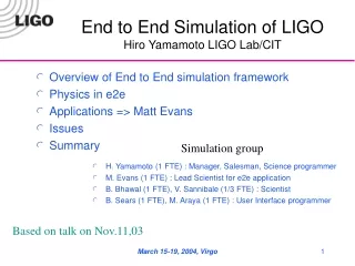
Built a simulator to understand characteristics of PSF and produce realistic images based on physics of the atmosphere, telescope, and detector Use a photon Monte Carlo approach (time-dependent and wavelength-dependent effects are straight-forward) Piece of UDF through 12 layers of atmosphere, complete LSST optics, and detector with complete wavelength dependent effects, fairly high fidelity in some areas, and does this in 1/2 hour
Overview of Simulator Structure Single photon MC approach in which every photon is followed from the sky (image+) Through atmosphere, Raytraced in optics to conversion/diffusion in the detector
Sky Interface Image Mode 1: Arbitrary number of images with a spectra or power law spectra Mode 2: Grids of stars with an Arbitrary spectraor power law spectra Maps and spectra are treated as lookup probability tables to draw photons Mode 3: Make synthetic stars and galaxies each with their own spectra + or power law Spectral Energy Distribution (SED)
Atmosphere Models: Kolmogorov turbulence: Energy cascades from largest to smallest scale having -11/3 spectrum Density (and therefore index of refraction) fluctuations follow velocity fluctuations Timescale for turbulence cascade >> (Windspeed)*(Exp. Time) size ==> frozen screen approximation with Kolmogorov statistics From Hardy 1998 (p.81)
Altitude Altitude Wind Speed Structure Function Can construct a model with layers with varying wind speeds and turbulence Vernin et al., Gemini RPT-A0-G0094 from Sebag
Atmosphere Interface and Raytrace LSST Aperture Vector Screen: 2048 squared 0.1m/pixel can have arbitrary number with arbitrary wind velocity vectors at given altitude Photons raytraced and shifted accordingly Optics
Optics Fast ray trace Calculates ray intercepts Uses reflection and refraction algorithms to compute the new ray trajectory Wavelength-dep index of refr. Have implemented 3.5 degree short tube design stored in pre-computed tables
Perturbations due to thermal and mechanical distortions Each optic has 6 dof (decenter, defocus, three euler angles) Perturbations are placed on the three mirrors using a Zernike (polynomials orthogonal on a circle) expansion to simulate the possible residual control system errors until the control system is simulated each mirror can have an arbitrary amplitude code goes up to 5th order polynomials This perturbation model will be replaced by control system residual estimation for body motions and zernikes
Detector: Refraction for light entering the Si surface Photon interaction (wavelength and temperature dependent) Lateral diffusion due to finite electric field
+Detector +Mirror Perturbations Optics (aberrations) ~2m, e~20% ~4m, e~20% ~10m, e~3% ~15m, e~0 to1% ~20m, e~2% ~20m, e~7% +Atmosphere Atmos+wind only +Wind
Complete end-to-end simulation of one chip of LSST/ 100 exposures