Download
1 / 64
640 likes | 783 Views
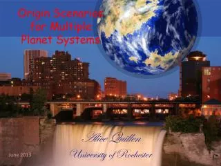
Origin Scenarios for Multiple Planet Systems. Alice Quillen University of Rochester. Conjunctions between Kep 36 planets . Conjunction every 97 days (7 times orbital period of inner planet or 6 times orbit of outer planet)

E N D
Origin Scenarios for Multiple Planet Systems Alice Quillen University of Rochester
Conjunctions between Kep 36 planets • Conjunction every 97 days (7 times orbital period of inner planet or 6 times orbit of outer planet) • Distance between planets at conjunction is 85 planet radii or 2 million km (about 5 times the distance between the Earth and Moon). • A viewer on planet b would see an angular diameter for planet c of 1.3 degrees. About 3 times larger than the Sun or Moon on the sky. Large size lasting a few days! • Angular Velocity on the sky (~1.5 degree/hour) with respect to the back ground stars is about 3 times faster than Moon as seen from the Earth
In collaboration with • Alex Moore • ImranHasan • Eva Bodman • Richard Edgar
Kepler ObservatorySearch for Planetary Transits in Light-curves (Carter et al. 2012) Kepler 36b Kepler 36c
The Kepler Multiple planet systems • Lower planet masses than Doppler (radial velocity discovered) planets • closely packed, short periods, compact systems • nearly circular orbits • low inclinations • Statistically significant number of planet pairs near or in resonance Kepler planet candidate pairs (Fabrycky et al. astroph 2012) number of pairs period ratio
Orbital resonance The ratio of orbital periods of two bodies are nearly equal to a ratio of small integers using mean motions (angular rotation rates) integrating to give a resonant angle
Three unique and very different multiple planet systems • Kepler 36 • two transiting super-Earth planets in nearby orbits, near the 7:6 resonance and with extreme density contrast around a solar mass subgiant • HR 8799 (discovered via optical imaging) • 4 massive super-Jovian planets, with a debris disk in a young system around an A star, 3 planets in a chain of mean motion resonances 4:2:1 • KOI 730 (Kepler candidate system) • 4 transiting super-Earth planets in a chain of mean motion resonances around a Solar type star, 8:6:4:3 commensurability
What do the resonant systems tell us about planetary system formation and evolution? • Resonant systems can be delicate constraints on asteroid/planetesimal belts that can nudge planets out of resonance • Resonances are narrow. Migration of planets allows capture into resonance constraints on migration processes • e.g.,work by Man-Hoi Lee 2002, Willey Kley 2004, and Hanno Rein 2012
Transit Timing Variations Figure: Agol et al. 2004 star + two planets Shift in location of center of mass of internal system causes a change in the time of the transit of outer planet • Length of a transit gives a measurement for the radius of a planet, not its mass. • Transit timing variations allow measurement of planet masses! • Compact or/and resonant transiting systems give measurable transit timing variations. Planetary sized masses can be confirmed. • Both planetary masses and radii are measured in the Kepler 36 system
Transit timing variations in the Kepler 36 system Kep 36c transits Kep 36b transits Fits to the transit timing make it possible to measure the masses of both planets TRANSIT NUMBER Carter et al. 2012
Mass Radius relation of Kepler planets Kepler 36c outer planet fluffball Other exoplanets blue, Kepler-11 pink, Kepler-18b gray, Kepler-20 b and c brown, GJ 1214bviolet, CoRoT-7b green, Kepler-10b orange, 55 Cnce Kepler planets have a wide distribution of densities and so compositions! Kepler 36b inner planet solid rock+iron! Carter et al. 2012
Larger sample TTV planet pairs Iron Hadden & Lithwick 2013 Rock density Water ttv phase radius
Kepler 36 system Carter et al. (2012) measured via astro-seismology • Two planets, near the 7:6 resonance • Large density contrast inner planet outer planet
Quantities in the Kepler 36 system • Ratio of orbital periods is 1.1733 (7/6=1.1667) • Distance between planets at conjunction is only 4.8 Hill radii! (Chaotic dynamics: Deck et al. 2012) • Planet sizes are large compared to volume: Integrations must check for collisions • Circular velocity is ~90 km/s
Problems with in-situ formation • Petrovich et al. 2013: can only approximately match period distribution near 3:2 resonance • Hanson & Murray 2013: cannot account for fraction of 1 planet systems • Swift et al. 2013 on Kepler 32 system: Extremely massive primordial disk required in M star compact multiple planet systems, planets exist at boundary of dust sublimation radius
Planetary Migration Scenarios • A planet embedded in a gas disk drives spiral density waves • Damps the planet’s eccentricity • The planet usually moves inwards • facilitates convergent migration and resonance capture planet Phil Armitage
Migration via Scattering Planetesimals • A planet can migrate as it ejects and scatters planetesimals • Facilitates divergent migration Pulling planets out of resonance or resonance crossing Kirsh et al. 2009 eccentricity/eH semi-major axis in AU
Stochastic migration Planet receives little random kicks • Due to density variations from turbulence in the gas disk (e.g., Ketchum et al. 2011) • Due to scattering with planetesimals (e.g., previously explored for Neptune by R. Murray-Clay and J. Hahn) Jake Simon
Mean motion Resonances Can be modeled with a pendulum-like Hamiltonian θ Resonant angle. Two types of motion, librating/oscillating in or out of resonance Level curves showing orbits expand Kepler Hamiltonian due to two-planet interactions This model gives: resonant width, strength, libration frequency, adiabatic limit, eccentricity variation in resonance, probability of capture
Dimensional Analysis on the Pendulum • H units cm2 s-2 • Action variable p cm2 s-1 (H=Iω) and ω with 1/s • a cm-2 • b s-1 • Drift rate db/dt s-2 • ε cm2 s-2 Ignoring the distance from resonance we only have two parameters, a,ε Only one way to combine to get momentum Only one way to combine to get time Distance to resonance
Sizescales on the Pendulum • Libration timescale ~ • Momentum variation in resonance • Distance to resonance • Adiabatic limit • Critical eccentricity set from momentum scale • Perturbation required to push system out of resonance set by momentum scale • Drift rate allowing capture set by adiabatic limit
Dimensional analysis on the Andoyer Hamiltonian • We only have two important parameters if we ignore distance to resonance • a dimension cm-2 • ε dimension cm2-k s-2-k/2 • Only one way to form a timescale and one way to make a momentum sizescale. • The square of the timescale will tell us if we are in the adiabatic limit • The momentum sizescale will tell us if we are near the resonance (and set critical eccentricity ensuring capture in adiabatic limit)
First order Mean motion resonances Two regimes: High eccentricity: We model the system as if it were a pendulum with Low eccentricity : Use dimensional analysis for Andoyer Hamiltonian in the low eccentricity limit dividing line dependent on dimensional eccentricity estimate Before resonance capture we work with the low eccentricity dimensions After resonance capture we work with the pendulum models.
Can the Kepler 36 system be formed with convergent migration? • Two planet + central star N-body integrations • Outer planet migrates damping is forced by adding a drag term in the integration • Eccentricity damping forced circularization using a drag term that depends on the difference in velocity from a circular orbit semi-major axes with peri and apoapses period ratio semi-major axes 4:3 resonance apsidal angle apsidal angle = 0 in resonance (see Zhou & Sun 2003, Beauge & Michtchenko, many papers) time
Drift rates and Resonant strengths • If migration is too fast, resonance capture does not occur • Closer resonances are stronger. Only adiabatic (slow) drifts allow resonance capture. • Can we adjust the drift rate so that 4:3, 5:4, 6:5 resonances are bypassed but capture into the 7:6 is allowed? • Yes: but it is a fine tuning problem. The difference between critical drift rates is only about 20%
Eccentricities and Capture secular oscillations • High eccentricity systems are less likely to capture • Can we adjust the eccentricities so that resonance capture in 4:3, 5:4, 6:5 resonances is unlikely but 7:6 possible? • No. Critical eccentricities differ by only a few percent. eccentricity jump due to 7:5 resonance crossing capture into 3:2 prevented by eccentricities period ratio semi-major axes resonances are bypassed because of eccentricities time Secular oscillations and resonance crossings make it impossible to adjust eccentricities well enough
Stochastic migration Rein(2013) accounts for distribution of period ratios of planet pairs using a stochastic migration model • Does stochastic migration allow 4:3, 5:4, and 6:5 resonances to be bypassed, allowing capture into 7:6 resonance? • Yes, sometimes (also see work by Pardekooper and Rein 2013) • Random variations in semi-major axes can sometimes prevent resonance capture in 4:3, 5:4, 6:5 resonances period ratio semi-major axes capture into 7:6! resonances bypassed time
Problems with Stochastic migration planets collide! • Stochastic perturbations continue after resonance capture • System escapes resonance causing a collision between the planets period ratio semi-major axes time
Problems with Stochastic migration • If a gas disk causes both migration and stochastic forcing, then planets will not remain in resonance • Timescale for escape can be estimated using a diffusive argument at equilibrium eccentricity after resonance capture • Timescale for migration is similar to timescale for resonance escape Disk must be depleted soon after resonance capture to account for a system in the 7:6 resonance --- yet another fine tuning problem • Density difference in planets not explained
Collisions are inevitable Kepler Planets are close to their star Consider Planet Mercury, closest planet to the Sun • Mercury has a high mean density of 5.43 g cm-3 Why? • Fractionation at formation (heavy condensates) • afterwards slowly, (evaporation) • afterward quickly (collision) • See review by Benz 2007 MESSENGER image
Giant Impact Origin of Mercury Grazing collision stripped the mantle, leaving behind a dense core that is now the planet Mercury (Benz et al. 2008)
Geometry of collisions Figures by Asphaug (2010) grazing collision direct collision hit and run, mantle stripping
impact angle envelope stripping Asphaug(2010) slow collisions fast collisions
Alternate scenarios/mechanisms for density variations Photoevaporation and atmospheric escape Owen & Wu 2013, Lopez & Fortney 2013 • Critically dependent on core mass. However: densities of Kepler planets are NOT strongly dependent onsemi-major axis(Hadden & Lithwick 2013) there are other processes affecting planetary density
Planetary embryos in a disk edge • ``Planet trap’’ + transition disk setting (e.g.,Terquem & Papaloizou 2007, Moeckel& Armitage 2012, Morbidelli et al. 2008, Liu et al. 2011) • We run integrations with two planets + 7 embryos (twice the mass of Mars) • no applied stochastic forcing onto planets, instead embryos cause perturbations • The outermost planet and embryos external to the disk edge are allowed to migrate Zhang & Zhou 2010 Embryos can lie in the disk here!
Integrations of two planets and Mars mass embryos embryos migrate inwards Collisions with inner planet. Potentially stripping the planet in place semi-major axes two planets encounter with embryos nudge system out of 3:2 resonance period ratio Integration ends with two planets in the 7:6 resonance and in a stable configuration inclinations time
Inner and outer planet swap locations Outer planet that had experienced more collisions becomes innermost planet another integration semi-major axes encounters with embryos nudge system out of 3:2, 5:4 resonances period ratio Integration ends with two planets in the 6:5 resonance and in a stable configuration inclinations time
another integration semi-major axes Final state can be a resonant chain like KOI 730 period ratio Integration ends with two planets in the 4:3 resonance and an embryo in a 3:2 with the outer planet If a misaligned planet existed in the Kepler 36 system it would not have been seen in transit inclinations time
Diversity of Simulation Outcomes • Pairs of planets in high j resonances such as 6:5 and 7:6. Appear stable at end of simulation • Pairs of planets in lower j resonances such as 4:3 • Resonant chains • Collisions between planets and between planets and embryos • Embryo passed interior to two planets and left there (possibly inside sublimation radius, as for innermost planet in Kep 32 system) Comments • Collisions affect planetary inclinations -- transiting objects are sensitive to this • A different kind of fine tuning: Numbers and masses of embryos. Outcome sensitive to collisions!
7:5 Some simulations gave two planets in 7:5 resonance. 7:5 is just inside the 3:2 resonance. In smooth or stochastic migration scenarios, it is extremely unlikely to avoid capture into the stronger first order 3:2 resonance yet allow capture in 7:5
Recent Discovery of two systems in the 7:5 James S. Jenkins, & MikkoTuomi Phase folded radial velocity curves for the pair of planets orbiting HD41248 (left)and GJ180 (right), with both inner and outer planets shown at the top andbottom. All data for HD41248 is from HARPS, whereas the red, blue,and green data points for GJ180 are taken from UVES, HARPS, and PFS.
Small inner planet within dust sublimation radius Kepler 32 system Swift et al. 2013
Properties of collisions between embryos and planets Accretion may still occur Number of collisions impacts on inner planet especially likely to cause erosion vimpact/vcircular
Collision angles Impacts are normal Impacts are grazing High velocity, grazing impacts are present in the simulation suggesting that collisions could strip the envelope of a planet Number of collisions Impact angle (degrees)
Kepler 36 and wide range of Kepler planet densities Both planet migration and collisions are perhaps happening during late stages of planet formation, and just prior to disk depletion …
Resonant Chains • Prior to the discovery of GL876 and HR8799, the only known multiple object system in a chain of mean motion resonances was Io/Europa/Ganymede • Each pair of bodies is in a two body mean motion resonance • Integer ratios between mean motions of each pair of bodies • Convergent migration model via tidal forces for Galilean satellites resonance
Resonant Chains • Systems in chains of resonances drifted there by convergent migration through interaction with a gaseous disk (e.g. Wang et al. 2012) • Scattering with planetesimals usually causes planet orbits to diverge and so leave resonance What constraints can resonant chain systems HR8799 and KOI730 give us on their post gaseous disk depletion evolution?
KOI 730 systemresonant chain Discovered in initial tally of multiple planet Kepler candidates (Lissauer et al. 2011) • Planet masses estimated from transit depths • Period ratios obey a commensurability 8:6:4:3 • Outer and inner pair in 4:3 resonance • Middle pair in 3:2