Download
1 / 33
330 likes | 448 Views
CoSSci High Performance Computing for Anthropology and the Social Sciences. Lukasz Lacinski 1 Presenter (ECSS, U Chicago) Douglas White 2 Presenter and PI Rachana Ananthakrishnan 1 (Future planning) Tom Uram 3 (ECSS developer year 1) Tolga Oztan 2 (Section on DEf Modeling)

E N D
CoSSci High Performance Computing for Anthropology and the Social Sciences Lukasz Lacinski1 Presenter (ECSS, U Chicago) Douglas White2 Presenter and PI Rachana Ananthakrishnan1 (Future planning) Tom Uram3 (ECSS developer year 1) Tolga Oztan2 (Section on DEf Modeling) Bob Sinkovits4 (Section on Cohesion Modeling) Paul Rodriguez4 (Section on Causal Modeling) Nancy Wilkins-Diehr4 (SDSC ECSS) 27 slides plus 2 live demos 2+20 minute and 10 min discussion 1University of Chicago 2University of California, Irvine 3Argonne National Labe 4San Diego Supercomputer Center
Outline: Lukasz • Motivation • Architecture • Gateway tools • Anthropology and Social Sciences • Gateway to Galaxy • Demo screencast • LiveDemo: How to Share Histories • LiveDemo: Complex Social Science Gateway • New work for new modeling approaches
Motivation Create a gateway to support researchers and students, without requiring them to understand underlying computational resources and how to use them. Research analysis performed with the gateway should be: • Accessible – users can easily specify parameters and run tools • Reproducible – input parameters and results are captured so that any user can repeat and understand any result as a complete computational analysis • Transparent – users share and publish analysis through on-line histories and clips of variables for model storage and reproduction of results
Architecture (1) • Web service Galaxy – scientific workflow, data integration and data and analysis persistence and publishing platform • Compute resources • 2 UCI virtual machines, one planned at Santa Fe Institute each with 2 cores of Xeon CPU • XSEDE cluster – Trestles 324 compute nodes, each with 4 AMD Magny-Cours CPUs (32 cores)
Architecture (2) End users UCI VMs CoSSci Gateway 2 Xeon cores each XSEDE Trestles 324 compute nodes 4 AMD Magny-Cours CPUs each http://socscicompute.ss.uci.edu/
Gateway tools • Can perform cross-cultural analysis on sixdifferent ethnological datasets with of 2,657 variables to date: SCCS – Standard Cross-Cultural Sample (n=186,v=2109) LRB – Lewis R. Binford’s forager data (n=339,v=506) WNAI – Western North American Indians (n=172,v=496) XC – merged variables above from EA cases (n=371,v=2657) EA – Ethnographic Atlas (n=1270,v=166) AWC (Atlas of World Cultures (n=557,v=166) • Use the Dow-Eff functions implemented in an R workspace. The functions estimate OLS, logit, and multinomial logit models, using multiple imputation to handle the problem of missing data, and network lag terms to handle Galton’s Problem.
Future work, through this fall, 2014 • Use the mkmapping package to generate world maps with convex hulls for autocorrelation clusters. • Improve color maps generated by the Rworldmap package. Reduce the ordinal categories to maximum 9 values and 9 corresponding coloring of nodes. • Add scaling to support the fv4scale and mkscale functions implemented in DEf01d R-workspace. • Extend information printed to output CVS files. live demo by Lukasz can begin here
instructional youtubes and options for VM and Galaxy Modeling: Gateway screenshot SKIPc
Windows for entering model variables andmodeling histories: Gateway screenshot SKIP
Outline: Doug • Anthropology and Social Sciences • Examples of Current Modeling (DEf: Dow and Eff functions) • Testing prior anthropological theories (e.g., Tolga Oztan) • (and the discovery process with new models, methods, manuals) • Ongoing: Predictive cohesion in Complex Social Networks (Bob Sinkovits) • Future work for new modeling approaches • Cutting edge: Install and use Libraries for Causal models • Testing New Procedures: Bayesian Network • Finding (Causal) Network Structure • Comparing two (Moral Gods) models • Trestles bootstraps, Paul Rodriguez SDSC • Does solving Galton’s Problem lead to different resuts?
Anthropology and Social Sciences • CoSSci tools provide great advantages toobservational sciences: Solution to the problem of greatly inflated significance tests with clustering, evolutionary histories, proximities of sample units – producing 50% or more spurious results Thus: Solveactual determinants of variation in cross-cultural variation in beliefs and behaviors Howevolutionary and economic processes are deeply embedded in culture – new fields like roots of economic development Links of ecology to human cultural behaviors Adjustments appropriate to archaeological and ethnographic data Understanding our human past basic to understanding our future • The databases analyzed by Dow-Eff functions, compensating for missing data and Galton’s Problem of nonindependence of cases, are essential in integrating physical and biological science understandings with anthropological, historical and social sciences.
e.g., Regression Diagnostics Examples of Current Modeling • Scores of models have been done as chapters for the Wiley Companion for Cross-Cultural Research and in the classroom -- for which CoSSci manuals are now available Weaknesses in this model are (1) Wald: some additional variables may be missing;(2) The error terms (residuals) are heteroskedastic and not normally distributed.
E.g., Anthropologists have assumed that if a couple lives with the wife’s family, the WiMo is likely to be avoided; if with the husband’s family the HuFa is avoided, and so on, but there is no such evidence in any of our data. Nor that avoidances of any sort arise from projection of incest taboos, or variants of the Oedipus complex. Good samples and the correct statistical methods have been lacking. • Tolga Oztan, using DEf and our databases, shows the first evidence that avoidance behaviors involving kin predict broader networks of cooperative behavior through new in-laws and predict the expansion of political alliances and population sizes up to the appearanceof formalized intercommunity government. The discovery here is that kin behavior is a key source of the development of cooperation in foragers, and probably in early human evolution.The data match Fred Eggan’s and Radcliffe-Brown’s descriptions of formalized kin avoidances as maintaining respectful distance rather than conflicts with in-laws. Testing prior anthropological theories
DEf Autocorrelation regression shows evolutionary development of types of Avoidances Frequency of shared predictors for different types of Avoidances
Avoidance theory is supported by the SCCS and WNAI data. We take the evidence of eventual declinein the co-evolution of Avoidances andgreater complexity to be due to the competition from other forms of integrative hierarchy with the expansion of political complexity. Matrilineality, which disperses matrilineage men, is also a predictor of avoidances and creates effective defense against raiding, again linking avoidances to extended kin networks. Avoidance relationships are not based on fear but on respect. Gift-giving following stability in a recent marriage often leads to cessation of Avoidance. All these features are key to understanding cooperativity in human societies, which operates through cohesiveness. more
Social networks: Cohesiveness • With Bob Sinkovits of SDSC, a second ECSS award aims to achieve new measurements for one of the most important and complex problems in network mathematics, that of large overlapping sets of nodes that are structurally cohesive in both multi-connectedness and separating clusters by removing nodes, two measures that were proven to be precisely equivalent by Menger’s theorem, a fundamental key to understanding cooperativity in networks. • These larger-scale network models lend a high level of predictability to sets of network science measures, which are often loosely defined and imprecise. Menger-based methods provide the tools for understanding how the larger contexts of human societies and their multilevel organizational entities give the network embedding for other phenomena. (They provide a potential for transforming our understanding of how complex networks act dynamically in today's globally networked world.)
Menger’s Theorem in a nutshell Number of vertex disjoint paths (no two simultaneous paths share a vertex) T T T S S S = Minimum number of vertices that need to be removed so that source and target are no longer connected
Pair-wise cohesion matrix • Element (i,j) of the pair-wise cohesion matrix (PCM) is the number of vertex disjoint paths between vertices i and j • Binarized PCM: mij ≥ k, then mij 1; otherwise mij 0 • Treat the binarized PCM as a connectivity matrix; cliques are upper bounds on the k-components • Pair-wise Cohesion matrix • Binarized PCM • Vertices (1,2,4,5) form a candidate 3-component
Tackling the co-author data set • Co-author data set obtained from sociology journals 1963-99 (vertices are authors, edges connect co-authors). 128,151 authors reduced to 29,462 by focusing on the largest bi-connected component 128,151 68,285 29,462 20,181 disjoint clusters w/ 2-48 vertices 25,822 biconnected clusters w/ 2-36 vertices
Constructing the PCM • Constructing the PCM is a lot of work. Can reduce the effort by a factor of more than 10x by using some clever techniques to fill in the 2s and 3s D1 D2 • Use 3-vertex separators to find 3s • Use 2-vertex separators to find 2s • Fill in remaining elements of PCM using more expensive algorithms from the iGraph library and using the power of parallel computing
Not quite done • The methods described above are a big step in the right direction, but the results are too inclusive and contain both the k-component and possibly other vertices(k-candidates) • Currently working on techniques to address these shortcomings • Construct a modified pair-wise cohesion that will lead to less-inclusive k-candidates • Identify vertices or sets of vertices within the k-candidate that can be rejected • The object here, using HPC, is to be able to move from analysis of small-scale networks to the very large scale of complex or contemporary networks.
Future work for new modeling approaches • In the first round of work on Cross-Cultural Anthropological Modeling, Aug 2012-Aug 2014, ECSS installed 4 successive improvements of R software by Mathematical Anthropologist Malcolm Dow and Comparative Econometrician Anthon Eff ending with DEf01, DEf01c, DEf01d and code for creating scales. • New work involving Paul Rodriguez@SDSC. These single-variable dependent models also provided networks of variables that were fully imputed, and analyzed on Trestles using the R library(bnlearn) for Bayesian graphical network models. Next: Paul Rodriguez • A second round, Aug 2014-2016, is proposed for Paul Rodriguez andTolga Oztan to develop these new modeling using Trestles HPC, illustrated in the next slidesfor the variables in White’sHighGods models. The other big problems tackled will be time series, Akaike Information Criterion (AiCc) multivariate modeling, andpath analysis with imputed variables, none of which are discussed here.
Testing New Procedures: Bayesian Network • Get probability tables (i.e. frequency counts) for all variables (i.e. nodes) • Consider Joint Probability over all configurations of variable values, e.g. P(HiGd,FxCmW,AnXbw,NoRnDry,Wrtng,v1695,v270,v1650) • Dependencies (edges) determine conditioning variables for each table, e.g. P(HiGod |AnXbwlth, No_Rn_Dry) = P(HiGod| AnXbwlth) Anxbw HiGod NoRnD
Finding Network Structure • Network Fit Measure For a given graph (i.e. dependencies), all frequency counts can be reproduced • Dependencies are given or discovered: all searching needs to score network on fit locally (are edges good) globally (is whole network good) greedy search or ‘hill climbing’ (heuristics guide search), BUT, many solutions with same fit Approach: using R package bnlearn with bootstrap samples to get network statistics (borrowing ideas from biological network discovery)
New Bayesian Network Learning Results with DEfimputed data and library(bnlearn) in comparing two Moral Gods models (left/right) Bayesian Network Learning Results p.13 Causal modeling (Trestles HPC) AnimXbwealth HiGod0 1 2 3 4 5 7 8 9 1 54 7 6 1 0 0 0 1 0 2 40 6 5 0 0 0 0 0 0 3 13 1 4 3 1 0 1 0 0 4 21 2 0 9 3 1 0 3 4 White, Oztan & Snarey (2014) Brown & Eff (2010) HiGod FxCmtyWages 1 2 3 4 0 43 27 11 17 1 18 11 5 23 3=not Islam or Christianity 4=supportive of morality Writing & Records HiGod1 2 3 4 5 1 35 16 10 0 8 2 25 17 6 0 3 3 7 9 3 2 2 4 6 7 2 10 18
1000 bootstrap resamples were taken by sampling the original dataset with replacement(only takes few minutes) For each new sample dataset, a bayes network was found using the grow-shrink algorithm The binary valued adjacency matrix was averaged across all 1000 networks Adjacency matrices were sorted and counted Trestles bootstraps, Paul Rodriguez SDSC, cont. 155 frequency 0 Unique Adjacency Matrices
Bioconductor.blocLite.R library(bootstrap) Paul Rodriguez SDSCblocLite(Rgraphviz)V=letters[1:10]M=1:4g1=randomGraph(V,M,0.2)plot(g1)Probabilities are generated by bootstrap, run on SDSC Trestles supercomputer 1695=No Scarification, 270=Class stratification
3rd-step regression with imputed variables: White et al (bold or red) vs. Brown & Eff Coefficients: Estimate Std. Error t value Pr(>|t|) (Intercept) 0.006272 0.473491 0.013 0.98945 Wy 0.651359 0.136649 4.767 0.00061 p<.001 FxCmtyWages* 0.751684 0.259420 2.898 0.00426 p<.01 + Missions 0.334426 0.140836 2.375 0.01868 p<.02 bio.5 (temp) -0.150861 0.079799 -1.891 0.06039 p<.10 PCsizeSq** -0.077855 0.041264 -1.887 0.06090 p<.01 Writing 0.115742 0.064661 1.790 0.07524 p<.01 Caste 0.171590 0.104619 1.640 0.10283 AnimXbwealth 0.090378 0.059296 1.524 0.12932 DistantFather -0.129960 0.087188 -1.491 0.13793 No_rain_Dry 0.120057 0.083832 1.432 0.15395 PCsize 0.102367 0.078573 1.303 0.19440 ExtWar -0.013503 0.010783 -1.252 0.21221 AgPot -0.053785 0.064506 -0.834 0.40556 FoodScarcity 0.018975 0.056114 0.338 0.73567 Anim -0.006878 0.057393 -0.120 0.90476 *The FxCmtyWages variable is, as hypothesized, significant. **Works in both models. All variables imputed for n=186
Estimate Std. Error t value Pr(>|t|) (Intercept) 1.019415 0.729651 1.397 0.16577 dx$FxCmtyWages 0.023184 0.273012 0.085 0.93251 <- n.s. dx$v2006 Missions 0.457471 0.220324 2.076 0.04068 P<.05 dx$v149 Writing 0.260651 0.104351 2.498 0.01429 p<.05 dx$v272 0.193109 0.182208 1.060 0.29203 dx$AnimXbwealth 0.105582 0.079593 1.327 0.18798 dx$v3 -0.003290 0.072426 -0.045 0.96387 dx$No_rain_Dry 0.340791 0.126310 2.698 0.00831 p<.01 dx$v1650 -0.012738 0.015911 -0.801 0.42546 dx$v1685 -0.038787 0.082818 -0.468 0.64066 dx$v206 -0.008370 0.072604 -0.115 0.90848 dx$bio.5 -0.002922 0.001762 -1.659 0.10064 PCAP 0.139448 0.101782 1.370 0.17404 PCsize 0.025052 0.140601 0.178 0.85898 PCsizeSq -0.054963 0.057641 -0.954 0.34284 In regard to autocorrelation, i.e., Galton’s problem, do our DEfresults differ from OLS? Yes, these are ols.
Contact Lukasz Lacinski lukasz@uchicago.edu Douglas White douglas.white@uci.edu
A bootstrap procedure was used to explore the distribution of possible network models (Efron & Tishbrini, 1986). One thousand bootstrap resamples were taken by sampling the original dataset with replacement. For each new sample dataset, a bayes network was found using the grow-shrink algorithm (heeding independencies in the data). The binary valued adjacency matrix for each network was saved and then averaged across all 1000 networks, thereby producing an expectation for the presence of every edge (Figure with graph in file named 'BNwboot_nowy_05thresh'). This approach has proved very useful in biological network discovery (e.g. Marbach, etal. 2012). The expectation serves as a weight on the edge, but it does not indicate what typical networks appear in the bootstrap samples. Therefore, we also sorted and counted the adjacency matrices, and printed out the most frequent networks. Efron, B.; Tibshirani, R. 1993. An Introduction to the Bootstrap. Chapman & Hall/CRC. Marbach D, Costello JC, Küffner R, Vega NM, Prill RJ, Camacho DM, Allison KR; The DREAM5 Consortium, Kellis M, Collins JJ, Stolovitzky G. 2012. Wisdom of crowds for robust gene network inference. Nature Methods9(8):796-804. 58 collaborators.Margaritis, D. and Thrun, S. 2000. Bayesian network induction via local neighborhoods. In Advances in Neural Information Processing Systems 12. (“the bootstrap.”) Trestles bootstraps, Paul Rodriguez SDSC SKIP