Download
1 / 21
280 likes | 649 Views
SIMULATION OF A SINGLE-SERVER QUEUEING SYSTEM. Will show how to simulate a specific version of the single-server queuing system Though simple, it contains many features found in all simulation models. 1- Problem Statement. Recall single-server queuing model

E N D
SIMULATION OF A SINGLE-SERVER QUEUEING SYSTEM • Will show how to simulate a specific version of the single-server queuing system • Though simple, it contains many features found in all simulation models
1- Problem Statement • Recall single-server queuing model • Assume interarrival times are independent and identically distributed (IID) random variables • Assume service times are IID, and are independent of interarrival times • Queue discipline is FIFO • Start empty and idle at time 0 • First customer arrives after an interarrival time, not at time 0 • Stopping rule: When nth customer has completed delay in queue (i.e., enters service) … n will be specified as input
1- Problem Statement (cont’d.) • Quantities to be estimated • Expected average delay in queue (excluding service time) of the n customers completing their delays • Why “expected?” • Expected average number of customers in queue (excluding any in service) • A continuous-time average • Area under Q(t) = queue length at time t, divided by T(n) = time simulation ends … see book for justification and details • Expected utilization (proportion of time busy) of the server • Another continuous-time average • Area under B(t) = server-busy function (1 if busy, 0 if idle at time t), divided by T(n) … justification and details in book • Many others are possible (maxima, minima, time or number in system, proportions, quantiles, variances …)
2- Intuitive Explanation • Given (for now) interarrival times (all times are in minutes): 0.4, 1.2, 0.5, 1.7, 0.2, 1.6, 0.2, 1.4, 1.9, … • Given service times: 2.0, 0.7, 0.2, 1.1, 3.7, 0.6, … • n = 6 delays in queue desired • “Hand” simulation: • Display system, state variables, clock, event list, statistical counters … all after execution of each event • Use above lists of interarrival, service times to “drive” simulation • Stop when number of delays hits n = 6, compute output performance measures
Interarrival times: 0.4, 1.2, 0.5, 1.7, 0.2, 1.6, 0.2, 1.4, 1.9, … Service times: 2.0, 0.7, 0.2, 1.1, 3.7, 0.6, … 2- Intuitive Explanation (cont’d) Status shown is after all changes have been made in each case …
Interarrival times: 0.4, 1.2, 0.5, 1.7, 0.2, 1.6, 0.2, 1.4, 1.9, … Service times: 2.0, 0.7, 0.2, 1.1, 3.7, 0.6, … 2- Intuitive Explanation (cont’d)
Interarrival times: 0.4, 1.2, 0.5, 1.7, 0.2, 1.6, 0.2, 1.4, 1.9, … Service times: 2.0, 0.7, 0.2, 1.1, 3.7, 0.6, … 2- Intuitive Explanation (cont’d)
Interarrival times: 0.4, 1.2, 0.5, 1.7, 0.2, 1.6, 0.2, 1.4, 1.9, … Service times: 2.0, 0.7, 0.2, 1.1, 3.7, 0.6, … 2- Intuitive Explanation (cont’d)
Interarrival times: 0.4, 1.2, 0.5, 1.7, 0.2, 1.6, 0.2, 1.4, 1.9, … Service times: 2.0, 0.7, 0.2, 1.1, 3.7, 0.6, … 2- Intuitive Explanation (cont’d)
Interarrival times: 0.4, 1.2, 0.5, 1.7, 0.2, 1.6, 0.2, 1.4, 1.9, … Service times: 2.0, 0.7, 0.2, 1.1, 3.7, 0.6, … 2- Intuitive Explanation (cont’d)
Interarrival times: 0.4, 1.2, 0.5, 1.7, 0.2, 1.6, 0.2, 1.4, 1.9, … Service times: 2.0, 0.7, 0.2, 1.1, 3.7, 0.6, … 2- Intuitive Explanation (cont’d)
Interarrival times: 0.4, 1.2, 0.5, 1.7, 0.2, 1.6, 0.2, 1.4, 1.9, … Service times: 2.0, 0.7, 0.2, 1.1, 3.7, 0.6, … 2- Intuitive Explanation (cont’d)
Interarrival times: 0.4, 1.2, 0.5, 1.7, 0.2, 1.6, 0.2, 1.4, 1.9, … Service times: 2.0, 0.7, 0.2, 1.1, 3.7, 0.6, … 2- Intuitive Explanation (cont’d)
Interarrival times: 0.4, 1.2, 0.5, 1.7, 0.2, 1.6, 0.2, 1.4, 1.9, … Service times: 2.0, 0.7, 0.2, 1.1, 3.7, 0.6, … 2- Intuitive Explanation (cont’d)
Interarrival times: 0.4, 1.2, 0.5, 1.7, 0.2, 1.6, 0.2, 1.4, 1.9, … Service times: 2.0, 0.7, 0.2, 1.1, 3.7, 0.6, … 2- Intuitive Explanation (cont’d)
Interarrival times: 0.4, 1.2, 0.5, 1.7, 0.2, 1.6, 0.2, 1.4, 1.9, … Service times: 2.0, 0.7, 0.2, 1.1, 3.7, 0.6, … 2- Intuitive Explanation (cont’d)
Interarrival times: 0.4, 1.2, 0.5, 1.7, 0.2, 1.6, 0.2, 1.4, 1.9, … Service times: 2.0, 0.7, 0.2, 1.1, 3.7, 0.6, … 2- Intuitive Explanation (cont’d)
Interarrival times: 0.4, 1.2, 0.5, 1.7, 0.2, 1.6, 0.2, 1.4, 1.9, … Service times: 2.0, 0.7, 0.2, 1.1, 3.7, 0.6, … 2- Intuitive Explanation (cont’d) Final output performance measures: Average delay in queue = 5.7/6 = 0.95 min./cust. Time-average number in queue = 9.9/8.6 = 1.15 custs. Server utilization = 7.7/8.6 = 0.90 (dimensionless)
3- Program Organization and Logic • C program to do this model (FORTRAN as well is in book) • Event types: 1 for arrival, 2 for departure • Modularize for initialization, timing, events, library, report, main • Changes from hand simulation: • Stopping rule: n = 1000 (rather than 6) • Interarrival and service times “drawn” from an exponential distribution (mean b = 1 for interarrivals, 0.5 for service times) • Density function • Cumulative distribution function
3- Program Organization and Logic (cont’d.) • How to “draw” (or generate) an observation (variate) from an exponential distribution? • Proposal: • Assume a perfect random-number generator that generates IID variates from a continuous uniform distribution on [0, 1] … • Algorithm: 1. Generate a random number U 2. Return X = – blnU • Proof that algorithm is correct:
ALTERNATIVE APPROACHES TO MODELING AND CODING SIMULATIONS • Parallel and distributed simulation • Various kinds of parallel and distributed architectures • Break up a simulation model in some way, run the different parts simultaneously on different parallel processors • Different ways to break up model • By support functions – random-number generation, variate generation, event-list management, event routines, etc. • Decompose the model itself; assign different parts of model to different processors – message-passing to maintain synchronization, or forget synchronization and do “rollbacks” if necessary … “virtual time” • Web-based simulation • Central simulation engine, submit “jobs” over the web • Wide-scope parallel/distributed simulation