Download
1 / 44
440 likes | 898 Views
Supply and Demand Models. Chapter 3,4. Laws of Supply and Demand. Supply and Demand Framework. A description of a market includes the quantity of goods that are sold in that market, Q , and the price, P , at which they are sold.

E N D
Supply and Demand Models Chapter 3,4
Supply and Demand Framework • A description of a market includes the quantity of goods that are sold in that market, Q, and the price, P, at which they are sold. • Outcomes in the market are a function of the laws of supply and demand
Law of Demand • Ceteris parabis, There is an inverse relationship between the price of a good and the quantity that consumers would like to purchase. Demand Curve Mathematical representation of Law of Demand • Demand Curve (Geometry) • Demand Function (Algebra) • Demand Schedule (Spreadsheet) What does Ceteris Parabis mean?
Law of Demand Two Explanations: • Substitution Effect – Goods purchased to satisfy needs but other goods (substitutes) may also do so. When price rises, consumers have an incentive to switch goods. • Income Effect – Consumers have a limited budget. When price of a major item goes up, less money for purchase of all items.
Demand Curve P D P2 P1 Q Q2 Q1
Demand Functions • An algebraic equation representing demand as a function of the price plus consumer income levels and other factors • Example:
Law of Supply: • Ceteris parabis, there is a positive relationship between the price of a good and the quantity producers bring to the market. Supply Curve Mathematical representation of Law of Supply • Supply Curve (Geometry) • Supply Function (Algebra) • Supply Schedule (Spreadsheet)
Law of Supply Explanation • Increasing Costs Producers will bring goods to market only if the price obtained from selling an extra good will exceed the cost of producing an extra good. If per unit production costs are rising in the number of goods produced, higher prices will be demanded to bring a larger quantity of goods to market.
Supply Curve P S P2 P1 Q Q1 Q2
Supply Functions • An algebraic equation representing supply as a function of the price plus input costs and other factors • Example:
Equilibrium • Equilibrium in the competitive market occurs when the price is set at a level (P*) such that the amount that consumers want to buy is equal to the amount that sellers want to sell (Q*). Excess SupplyIf P were above equilibrium, sellers would want to sell more goods than buyers would want to buy. Competition between sellers would force prices down. Excess DemandIf P were below equilibrium, customers would want to buy more goods than people would want to sell. Competition between buyers would force prices up.
Competitive Market Equilibrium P S D 1 P* Q* Q
Excess Supply P S D P* Q* Q
Excess Demand P S D P* Q* Q
Market Equilibrium(Spreadsheet Problem) At what price and quantity (to closest $10) will the oil market clear?
To think about commodity prices, economists first think about the theory of competitive markets • Competitive Markets have many buyers and many sellers who compete without barriers preventing rivals from entering or leaving the market. • Participants in competitive markets are price takers, agents who behave as if their own behavior has no effect on market prices.
Shifting Curves/Changing Equilibrium • Changes in equilibrium result from shifts in either the demand or supply schedule. We think of shifts in the curves as changes in supply or demand that are caused by factors other than changes in the price of the good. • Shifts in the demand curve lead to movements along the supply curve resulting in changes in prices and quantities that move in the same direction. • Shifts in the supply curve lead to movements along the demand curve resulting in changes in prices and quantities that move in different directions.
A Shift in the Demand Curve: A parallel increase in the demand schedule at every price point.Price and Quantity Demanded move in same direction P S Shift in the demand curve P** D′ P* D Q* Q** Q
A Shift in the Supply Curve is a Movement along the Demand curve- Price and Quantity Supplied Move in opposite Directions P S′ S D P** P* Q** Q* Q
Equilibrium Effects • Price system means that shifts in demand will cause changes in quantity supplied but also an attenuating change in quantity demanded. • Shifts in supply will cause changes in quantity demanded but also attenuating change in quantity supplied.
A Shift in the Demand Curve: Equilibrium Effect: Movement along the supply curve increases quantity supplied; movement along demand curve ameliorates quantity demanded. S P Along demand curve Along supply curve P** P* D′ D Q* Q** Q
A Shift in the Supply Curve: Equilibrium Effect: Movement along the demand curve reduces quantity demanded; movement along supply curve ameliorates quantity supplied. D S P S′ Along supply curve P** Along demand curve P* Q** Q* Q
Price Sensitivity and Equilibrium Effects • When supply or demand curve shifts, the effect will be felt in some combination of changes in prices and quantities. • The degree to which changes in either supply or demand are felt in quantity changes rather than price changes is determined by price sensitivity of both demand and supply.
Algebra of Supply and Demand • Linear Functions Parameters s and d denote the sensitivity of quantity demanded or quantity supplied to price changes.
Linear Functions – Described by Intercept (AS or AD ) and slope (1/s or 1/d). P S P* ,Q* 1 1 d 1 s D Q
What price sets supply equal to demand? • What quantity will be demanded (supplied) at hat price?
Algebra of Equilibrium Effects • If s or d are big, effects of supply or demand change on equilibrium price will be small • Effects of supply or demand changes on equilibrium quantity will be determined by relative price sensitivity.
Steeper (less price sensitive) supply curve means that a demand shift will have a smaller impact on quantity and bigger impact on price. . S1 P S2 1 P1** 2 P2** 0 P* D’ D Q Q* Q1** Q2**
Steeper (less elastic) demand curve means that a supply shift will have a smaller impact on quantity and bigger impact on price. . S’ P S 1 P1** 2 P2** 0 P* D2 D1 Q Q1** Q* Q2**
Steeper (less price sensitive) supply curve means that a supply shift will have a bigger impact on quantity and bigger impact on price. . S1 S1' P S2 S2' P* 0 P2** 2 P1** 1 D Q Q* Q2** Q1**
Steeper (less price sensitive) demand curve means that a demand shift will have a bigger impact on quantity and a bigger impact on price. . S’ P S P1** 2 1 P2** 0 P* D2 D2 D1 D1 Q Q1** Q* Q2**
Measuring the Impact of Price on Quantity Demanded • A natural way of measuring impact of a price change is to measure the change in quantity demanded relative in size to the change in prices.
Economists often prefer elasticity to slope in real world • This measure is the inverse of the SLOPE of the demand curve which is constant when the demand curve is linear (as often depicted in textbooks) • Economists typically do not measure the price impact using slope for 2 reasons. • Slope as a measure is not unit free, so price impacts are not comparable across types of goods or currency. • Empirical demand curves tend not to have constant slope or constant elasticity, but constant elasticity functions are a better approximation.
Price Elasticity:The % impact on quantity demanded of a 1% change in price
Midpoint Method • If you want to calculate a % difference between two points which is the same regardless of which you designate as the reference point (denominator), you can use the average of the two points as the reference point.
Learning Outcomes • Solve for equilibrium price and quantities using graphical supply and demand model or spreadsheet supply and demand schedules or simple linear algebra. • Explain qualitatively the likely consequences for equilibrium prices and quantities resulting from exogenous shifts in supply and demand. • Calculate elasticities using the midpoint method.