Download
1 / 7
70 likes | 374 Views
Second-Order Circuits Cont’d. Dr. Holbert April 24, 2006. Important Concepts. The differential equation for the circuit Forced (particular) and natural (complementary) solutions Transient and steady-state responses 1st order circuits: the time constant ( )

E N D
Second-Order Circuits Cont’d Dr. Holbert April 24, 2006 ECE201 Lect-22
Important Concepts • The differential equation for the circuit • Forced (particular) and natural (complementary) solutions • Transient and steady-state responses • 1st order circuits: the time constant () • 2nd order circuits: natural frequency (ω0) and the damping ratio (ζ) ECE201 Lect-22
Building Intuition • Even though there are an infinite number of differential equations, they all share common characteristics that allow intuition to be developed: • Particular and complementary solutions • Effects of initial conditions • Roots of the characteristic equation ECE201 Lect-22
Second-Order Natural Solution • The second-order ODE has a form of • To find the natural solution, we solve the characteristic equation: • Which has two roots: s1 and s2. ECE201 Lect-22
Step-by-Step Approach • Assume solution (only dc sources allowed): • x(t) = K1 + K2 e-t/ • x(t) = K1 + K2 es1t + K3 es2t • At t=0–, draw circuit with C as open circuit and L as short circuit; find IL(0–) and/or VC(0–) • At t=0+, redraw circuit and replace C and/or L with appropriate source of value obtained in step #2, and find x(0)=K1+K2 (+K3) • At t=, repeat step #2 to find x()=K1 ECE201 Lect-22
Step-by-Step Approach • Find time constant (), or characteristic roots (s) • Looking across the terminals of the C or L element, form Thevenin equivalent circuit; =RThC or =L/RTh • Write ODE at t>0; find s from characteristic equation • Finish up • Simply put the answer together. • Typically have to use dx(t)/dt│t=0 to generate another algebraic equation to solve for K2 & K3 (try repeating the circuit analysis of step #5 at t=0+, which basically means using the values obtained in step #3) ECE201 Lect-22
Class Examples • Learning Extension E7.10 • Learning Extension E7.11 ECE201 Lect-22