Download
1 / 49
500 likes | 824 Views
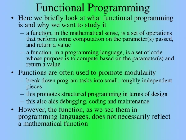
Functional Programming. Big Picture. What we’ve learned so far: Imperative Programming Languages Variables, binding, scoping, reference environment, etc What’s next: Functional Programming Languages Semantics of Programming Languages Control Flow Data Types Logic Programming

E N D
Big Picture • What we’ve learned so far: • Imperative Programming Languages • Variables, binding, scoping, reference environment, etc • What’s next: • Functional Programming Languages • Semantics of Programming Languages • Control Flow • Data Types • Logic Programming • Subroutines, Procedures: Control Abstraction • Data Abstraction and Object-Orientation
Design of Programming Languages • Design of imperative languages is based directly on the von Neumann architecture • Efficiency is the primary concern, rather than the suitability of the language for software development • Other designs: • Functional programming languages • Based on mathematical functions • Logic programming languages • Based on formal logic (specifically, predicate calculus)
Design View of a Program • If we ignore the details of computation (“how” of computation) and focus on the result being computed (“what” of computation) • A program becomes a “black box” for obtaining output from input Input Program Output
Functional Programming Language • Functional programming is a style of programming in which the primary method of computation is the application of functions to arguments x f(x) y Output Argument or variable Function
Historical Background 1940s: Alonzo Church and Haskell Curry developed the lambda calculus, a simple but powerful mathematical theory of functions. 6
Historical Background 1960s: John McCarthy developed Lisp, the first functional language. Some influences from the lambda calculus, but still retained variable assignments. 7
Historical Background 1978: John Backus publishes award winning article on FP, a functional language that emphasizes higher-order functions and calculating with programs. 8
Historical Background Mid 1970s: Robin Milner develops ML, the first of the modern functional languages, which introduced type inference and polymorphic types. 9
Historical Background Late 1970s - 1980s: David Turner develops a number of lazy functional languages leading up to Miranda, a commercial product. 10
Historical Background 1988: A committee of prominent researchers publishes the first definition of Haskell, a standard lazy functional language. 11
Historical Background 1999: The committee publishes the definition of Haskell 98, providing a long-awaited stable version of the language. 12
Basic Idea of Functional Programming • Think of programs, procedures and functions as being represented by the mathematical concept of a function • A mathematical function: {elts in domain} → {elts in range} • Example: sin(x) • domain set: set of all real numbers • range set: set of real numbers from –1 to +1 • In mathematics, variables always represent actual values • There is no such thing as a variable that models a memory location • Since there is no concept of memory location or l-value of variables, a statement such as (x = x + 1) makes no sense • A mathematical function defines a value, rather than specifying a sequence of operations on values in memory
Imperative Programming Summing the integers 1 to 10 in Java: total = 0; for (i = 1; i 10; ++i) total = total + i; The computation method is variable assignment Each variable is associated with a memory location 14
Functional Programming Summing the integers 1 to 10 in Haskell: sum [1..10] The computation method is function application. 15
Functional Programming • Function definition vs function application • Function definition • Declaration describing how a function is to be computed using formal parameters • Function application • A call to a declared function using actual parameters or arguments • In mathematics, a distinction is often not clearly made between a variable and a parameter • The term independent variable is often used for both actual and formal parameters
Functional Programming Language • The objective of the design of a FPL is to mimic mathematical functions to the greatest extent possible • Imperative language: operations are completed and results are stored in variables for later use • Management of variables is source of complexity for imperative programming • FPL: variables are not necessary • Without variables, iterative constructs are impossible • Repetition must be provided by recursion rather than iterativeconstructs
Example: GCD • Find the greatest common divisor (GCD) between 12 and 30 • Divisors for 12: 1, 2, 3, 4, 6, 12 • Divisors for 30: 1, 2, 3, 5, 6, 10, 15, 30 • GCD(12, 30) is equal to 6 • Algorithm: • u=30, v=12 30 mod 12 = 6 • u=12, v=6 12 mod 6 = 0 • u=6, v=0 since v=0, GCD=u=6
int gcd(int u, int v) { int temp; while (v != 0) { temp = v; v = u % v; u = temp; } return u; } * Computing GCD using iterative construct int gcd(int u, int v) { if (v==0) return u; else return gcd(v, u % v); } * Computing GCD using recursion Computing GCD
Fundamentals of FPLs • Referential transparency: • In FPL, the evaluation of a function always produces the same result given the same parameters • E.g., a function rand, which returns a (pseudo) random value, cannot be referentially transparent since it depends on the state of the machine (and previous calls to itself) • Most functional languages are implemented with interpreters
Using Imperative PLs to support FPLs • Limitations • Imperative languages often have restrictions on the types of values returned by the function • Example: in Fortran, only scalar values can be returned • Most of them cannot return functions • This limits the kinds of functional forms that can be provided • Functional side-effects • Occurs when the function changes one of its parameters or a global variable
Characteristics of Pure FPL • Pure FP languages tend to • Have no side-effects • Have no assignment statements • Often have no variables! • Be built on a small, concise framework • Have a simple, uniform syntax • Be implemented via interpreters rather than compilers
Functional Programming Languages • FPL provides • a set of primitive functions, • a set of functional forms to construct complex functions, • a function application operation, • some structure to represent data • In functional programming, functions are viewed as values themselves, which can be computed by other functions and can be parameters to other functions • Functions are first-class values
Lambda Expressions • Function definitions are often written as a function name, followed by list of parameters and mapping expression: • Example: cube (x) x * x * x • A lambda expression provides a method for defining nameless functions (x) x * x * x • Nameless functions are useful, e.g., functions that are produced for intermediate application to a parameter list do not need a name, for it is applied only at the point of its construction
Lambda Expressions • Function application • Lambda expressions are applied to parameter(s) by placing the parameter(s) after the expression e.g. ((x) x * x * x)(3) evaluates to 27 • Lambda expressions can have more than one parameter e.g. (x, y) x / y
Functional Forms • A functional form, is a function that either • takes functions as parameters, • yields a function as its result, • or both • Also known as higher-order function • Function Composition: • A functional form that takes two functions as parameters and yields a function whose result is a function whose value is the first actual parameter function applied to the result of the application of the second Example: h f ° g which means h (x) f ( g ( x)) If f(x) x + 2, g(x) 3 * x, then h(x) (3 * x) + 2
Functional Forms • Construction: A functional form that takes a list of functions as parameters and yields a list of the results of applying each of its parameter functions to a given parameter For f (x) x * x * x and g (x) x + 3, [f, g] (4) yields (64, 7) • Apply-to-all: A functional form that takes a single function as a parameter and yields a list of values obtained by applying the given function to each element of a list of parameters For h (x) x * x * x, ( h, (3, 2, 4)) yields (27, 8, 64)
LISP • Stands for LISt Processing • Originally, LISP was a typeless language and used for symbolic processing in AI • Two data types: • atoms (consists of symbols and numbers) • lists (that consist of atoms and nested lists) • LISP lists are stored internally as single-linked lists • Lambda notation is used to specify nameless functions (function_name (LAMBDA (arg_1 … arg_n) expression))
LISP • Function definitions, function applications, and data all have the same form • Example: • If the list (A B C) is interpreted as data, it is a simple list of three atoms, A, B, and C • If it is interpreted as a function application, it means that the function named A is applied to the two parameters, B and C • This uniformity of data and programs gives functional languages their flexibility and expressive power • programs can be manipulated dynamically
LISP • The first LISP interpreter appeared only as a demonstration of the universality of the computational capabilities of the notation • Example (early Lisp): (defun fact (n) (cond ((lessp n 2) 1)(T (times n (fact (sub1 n)))))) • The original intent was to have a notation for LISP programs that would be as close to Fortran’s as possible, with additions when necessary • This notation was called M-notation, for meta-notation • McCarthy believed that list processing could be used to study computability, which at the time was usually studied using Turing machines • McCarthy thought that symbolic lists was a more natural model of computation than Turing machines • Common Lisp is the ANSI standard Lisp specification • All LISP structures, including code and data, have uniform structure • Called S-expressions
LISP • EVAL: a universal function that could evaluate any other functions • LISP 1.5: • Awkward—though elegantly uniform—syntax. • Dynamic scope rule • Inconsistent treatment of functions as arguments—because of dynamic scoping
Scheme • A mid-1970s dialect of LISP, designed to be cleaner, more modern, and simpler version than the contemporary dialects of LISP • Uses only static scoping • Functions are first-class entities • They can be the values of expressions and elements of lists • They can be assigned to variables and passed as parameters
Scheme • Arithmetic: +, -, *, /, ABS, SQRT (+ 5 2) yields 7 • Most interpreters use prefix notations: • (+ 3 5 7) means add 3, 5, and 7 • (+ (* 3 5) (- 10 6)) • Advantages: • Operator/function can take arbitrary number of arguments • No ambiguity, because operator is always the leftmost element and the entire combination is delimited by parentheses
Scheme • QUOTE • takes one parameter; returns the parameter without evaluation • QUOTE is required because the Scheme interpreter, named EVAL, always evaluates parameters to function applications before applying the function. • QUOTE is used to avoid parameter valuation when it is not appropriate • QUOTE can be abbreviated with the apostrophe prefix operator • '(A B) is equivalent to (QUOTE (A B)) • (list a b c) versus (list 'a 'b 'c)
Scheme - • LIST takes any number of parameters; returns a list with the parameters as elements • CAR takes a list parameter; returns the first element of that list • (CAR '(A B C)) yields A • (CAR '((A B) C D)) yields (A B) • CDR takes a list parameter; returns the list after removing its first element • (CDR '(A B C)) yields (B C) • (CDR '((A B) C D)) yields (C D) • CONS returns a new list that includes the first parameter as its first element and the second parameter as remainder of its result • (CONS ’(A D) '(B C)) returns ((A D) B C)
Scheme: Predicate Functions • #T and () are true and false respectively • EQ? returns #T if both parameters are atoms and are the same • (EQ? 'A 'A) yields #T • (EQ? 'A '(A B)) yields () • Note that if EQ? is called with list parameters, the result is not reliable • Also, EQ? does not work for numeric atoms • LIST? returns #T if the parameter is a list; otherwise () • NULL? returns #T if the parameter is an empty list; otherwise () • Note that NULL? returns #T if the parameter is () • Numeric Predicate Functions=, <>, >, <, >=, <=, EVEN?, ODD?, ZERO?
Lambda Expressions • Form is based on notation • (LAMBDA (L) (CAR (CDR L))) • L is called a bound variable • Lambda expressions can be applied • ((LAMBDA(L) (CAR (CDR L))) '((A B) C D))
Constructing Functions • DEFINE - Two forms: • To bind a symbol to an expression • (DEFINE pi 3.141593) • (DEFINE two_pi (* 2 pi)) • To bind names to lambda expressions • (DEFINE (cube x) (* x x x)) • then you can use: (cube x)
Evaluation Process • Evaluation process (for normal functions): • Parameters are evaluated, in no particular order • The values of the parameters are substituted into the function body • The function body is evaluated • The value of the last expression in the body is the value of the function
Control Flow • Selection- the special form, IF • (IF predicate then_exp else_exp) • (IF (<> count 0) (/ sum count) 0 ) (DEFINE (factorial n) ( IF ( = n 0) 1 (* n (factorial(- n 1) ) ) ) )
Control Flow • Multiple Selection - the special form, COND (COND (predicate_1 expr {expr}) (predicate_1 expr {expr}) ... (predicate_1 expr {expr}) (ELSE expr {expr}) ) • Returns the value of the last expr in the first pair whose predicate evaluates to true
Example Scheme Function • member • takes an atom and a list; • returns #T if atom is in list; () otherwise (DEFINE (member atm lis) (COND ((NULL? lis) '()) ((EQ? atm (CAR lis)) #T) ((ELSE (member atm (CDR lis))) ))
Example Scheme Function • equalsimp • returns #T if the two simple lists are equal; () otherwise (DEFINE (equalsimp lis1 lis2) (COND ((NULL? lis1) (NULL? lis2)) ((NULL? lis2) '()) ((EQ? (CAR lis1) (CAR lis2)) (equalsimp (CDR lis1) (CDR lis2))) (ELSE '()) ))
Example Scheme Function • equal • returns #T if the two general lists are equal; () otherwise (DEFINE (equal lis1 lis2) (COND ((NOT (LIST? lis1)) (EQ? lis1 lis2)) ((NOT (LIST? lis2)) '()) ((NULL? lis1) (NULL? lis2)) ((NULL? lis2) '()) ((equal (CAR lis1) (CAR lis2)) (equal (CDR lis1) (CDR lis2))) (ELSE '()) ))
Example Scheme Function • Append • takes two lists as parameters; returns the first parameter list with the elements of the second parameter list appended at the end (DEFINE (append lis1 lis2) (COND ((NULL? lis1) lis2) (ELSE (CONS (CAR lis1) (append (CDR lis1) lis2))) ))
Scheme Functional Forms • Composition • The previous examples have used it • Apply to All • one form in Scheme is mapcar • Applies the given function to all elements of the given list; result is a list of the results (DEFINE mapcar fun lis) (COND ((NULL? lis) '()) (ELSE (CONS (fun (CAR lis)) (mapcar fun (CDR lis)))) ))
EVAL • Scheme interpreter itself is a function named EVAL • The EVAL function can also be called directly by Scheme programs • It is possible for Scheme to create expressions and calls EVAL to evaluate them • Example: adding a list of numbers • Cannot apply “+” directly on a list because “+” takes any number of numeric atoms as arguments • (+ 1 2 3 4) is OK • (+ (1 2 3 4)) is not
EVAL • One approach: ((DEFINE (adder lis) (COND ((NULL? lis) 0) (ELSE (+ (CAR lis) (adder (CDR lis)))) • Another approach: ((DEFINE (adder lis) (COND ((NULL? lis) 0) (ELSE (EVAL (CONS '+ lis))) )) • (adder ‘(3 4 6)) causes adder to build the list (+ 3 4 6) • The list is then submitted to EVAL, which invokes + and returns the result 13
Scheme: Output Functions • Output Utility Functions: • (DISPLAY expression) • Example: (DISPLAY (car ‘(A B C))) • (NEWLINE)