Download
1 / 21
210 likes | 349 Views
Statistical Reasoning for everyday life. Intro to Probability and Statistics Mr. Spering – Room 113. 3.2 Picturing Distributions of Data.

E N D
Statistical Reasoningfor everyday life Intro to Probability and Statistics Mr. Spering – Room 113
3.2 Picturing Distributions of Data • Distribution – refers to the way in which values are spread over all possible values. We can summarize a distribution in a table or show a distribution visually with a graph. • {i.e. bar graph, histogram, pareto chart, dot plot, pie chart, stem-and-leaf plot, line chart, time-series diagram, scatter plot, and box-whisker plot (review in section 4.3)}
3.2 Picturing Distributions of Data • (Crucial Components) Important Labels for Graphs • Vertical scale – numbers along the vertical axis should clearly indicate the scale. The numbers should line up with the tick marks – the marks along the axis that precisely locate the numerical values. • Horizontal scale – the categories should be clearly indicated along the horizontal axis (Tick marks may not be necessary for qualitative data, but should be included for quantitative data.) • Vertical axis title – Include a title that describes the variable shown on the vertical axis • Horizontal axis title – Include a title that describes the variable shown on the horizontal axis • Title/caption and legend (key) – the graph should have a title or caption that explains what is being shown, and if applicable, lists the source of the data. If multiple data sets are displayed on a single graph, include a legend or key to identify the individual data sets.
3.2 Picturing Distributions of Data • Bar graph – is a diagram consisting of bars that represent the frequencies (or relative frequencies) for particular categories. The lengths of the bars are proportional to the frequency. • EXAMPLE: • Number of police officers in Crimeville, 1993 to 2001
3.2 Picturing Distributions of Data • Dot plot (line plot) – similar to a bar graph, except each individual data value is represent by a dot or symbol. • EXAMPLE: Barley Yields, Grand Rapids
3.2 Picturing Distributions of Data • Pareto chart – is a bar graph with the bars arranged in order according to frequency. Pareto charts make sense only for data at the nominal level of measurement.
3.2 Picturing Distributions of Data • Pie Chart (circle graph) – circle divided so that each wedge represents that relative frequency of a particular category. The wedge size is proportional to the relative frequency and 360 degrees. The entire pie represents the total relative frequency of 100%. • Example: Music preferences in young adults 14 to 19
3.2 Picturing Distributions of Data • Histogram – is a bar graph showing a distribution for quantitative data (at the interval or ratio level); the bars have a natural order and the bar widths have specific meaning. • EXAMPLE: Exam Scores of 27 students
3.2 Picturing Distributions of Data • Stem-and-leaf plot – much like a histogram turned sideways, except in place of bars we see a listing of the individual data sources or values. {Allows us to list all data easily} • Example: The numbers 40, 42, and 43 are from Data Set A.The numbers 41, 45, 46, and 47 are from Data Set B.
3.2 Picturing Distributions of Data • Line chart (line graph) – shows distribution of quantitative data as a series of dots connected by lines. Each dot is the center of the bin it represents and the vertical position is the frequency value for the bin. {Line charts help us to see increasing and decreasing trends.} • Example:
3.2 Picturing Distributions of Data • Scatter plot – is a chart that uses Cartesian coordinates to display values for two variables. The data is displayed as a collection of points, each having one coordinate on the horizontal axis and one on the vertical axis. • A scatter plot does not specify dependent or independent variables. Either type of variable can be plotted on either axis. Scatter plots represent the association (not causation) between two variables.
3.2 Picturing Distributions of Data • Time-series diagram (plots over time) – A histogram or line chart in which the horizontal axis represents time. NEXT SLIDE…
3.2 Picturing Distributions of DataEXAMPLE: Time-series diagram
3.2 Picturing Distributions of Data • Summary: Many different ways to display data. Remember be very observant, and study displays carefully for misleading information. Finally, make sure you can recognize and interpret all forms of display.
3.2 Picturing Distributions of Data GOOD LUCK !!!!!!!
3.2 Picturing Distributions of Data How many degrees hotter was it on Wednesday than Thursday? 30-10=20 degrees hotter
3.2 Picturing Distributions of Data Data from an experiment was put into a circle graph and a bar graph. Which set of bars could show the same data as the circle graph?
3.2 Picturing Distributions of Data A band director surveyed her students to ask them their favorite instrument. The table shows the results of the survey. Which is the most appropriate graph of the information in the table to show what fraction of the students choose each instrument?
3.2 Picturing Distributions of Data The following stem-and-leaf plot shows the ages of the teachers at Central Heights Elementary School. Which age group has the most teachers? KEY: 4 | 5 = 45 Teachers in their thirties
3.2 Picturing Distributions of Data The graph shows the population of four towns. • Town A • Town D • Left out important/relevant information
3.2 Picturing Distributions of Data • HW: pg 110 # 1, 5 – 14 all, 19, 21, 25