Download
1 / 34
350 likes | 514 Views
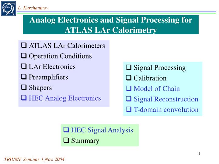
ATLAS LAr Calorimeters Operation Conditions LAr Electronics Preamplifiers Shapers HEC Analog Electronics. L. Kurchaninov. TRIUMF Seminar 1 Nov. 200 4. Analog Electronics and Signal Processing for ATLAS LAr Calorimetry. Signal Processing Calibration Model of Chain

E N D
ATLAS LAr Calorimeters Operation Conditions LAr Electronics Preamplifiers Shapers HEC Analog Electronics L. Kurchaninov TRIUMF Seminar1 Nov. 2004 Analog Electronics and Signal Processing for ATLAS LAr Calorimetry • Signal Processing • Calibration • Model of Chain • Signal Reconstruction • T-domain convolution • HEC Signal Analysis • Summary
L. Kurchaninov TRIUMF Seminar1 Nov. 2004 ATLAS LAr Calorimeters: 3 technologies
L. Kurchaninov TRIUMF Seminar1 Nov. 2004 ATLAS LAr Calorimeters: Accordion LAr gap: ~2mm Almost uniform electric field, charge collection as in parallel-plate chamber Drift time ~400 - 500 ns Cd = 200 – 2000 pF
L. Kurchaninov TRIUMF Seminar1 Nov. 2004 ATLAS LAr Calorimeters: HEC Parallel-plate ionization chamber with EST electrodes LAr gap: ~4x2mm, drift time ~450 ns Cd = 50 – 450 pF
L. Kurchaninov FEB TRIUMF Seminar1 Nov. 2004 ATLAS LAr Calorimeters: FCAL LAr gap: 0.25 - 0.375 - 0.5 mm Drift time: 50 – 75 – 100 ns Cd = 1000 – 1500 pF
L. Kurchaninov TRIUMF Seminar1 Nov. 2004 Operation Conditions: LHC Bunches LHC bunch crossing (BC) period 24.96 ns Readout is synchronized with LHC clock LAr signals are digitized each BC
L. Kurchaninov TRIUMF Seminar1 Nov. 2004 Operation Conditions: Pileup Interactions each BC ~ 23 “minimum bias” events for full luminocity • Pileup of signals from past bunch crossings • Pilup noise in addition to electronic noise • Pedestal modulation due to non-regular bunch structure Not negligible for high h region
L. Kurchaninov Digitization and optical output 144-cells analog memory Three gain RC2-CR shaper Warm hybrid preamplifiers (preshapers for HEC) Passive cold electronics (active for HEC) TRIUMF Seminar1 Nov. 2004 LAr Electronics: Archeticture
L. Kurchaninov TRIUMF Seminar1 Nov. 2004 LAr Electronics: Front-End Board 128 input channels, 32 trigger output channels 16 ADCs, 1 optical output Daughter boards: 32 preamp (preshaper), LSB 8 ASICs Production (1611 FEBs) started
L. Kurchaninov TRIUMF Seminar1 Nov. 2004 Preamplifiers: Technology Choice Low noise .. Low power .. Fast .. Rad hard .. Low Zin .. GaAs FET (cold) vs. Bipolar transistor (warm) HEC: GaAs – not so many channels, enough room for preamps EMB, EMEC: Bipolar – less dead material, no power in cryostat FCAL: Bipolar – radiation levels
L. Kurchaninov TRIUMF Seminar1 Nov. 2004 Preamplifies: Requirements and Design Wide range of Cd Zin = 50 or 25 W to match cables Different range of input signals in EM and FCAL Radiation hardness HV protection
L. Kurchaninov TRIUMF Seminar1 Nov. 2004 Shapers: Choice and Optimization RC2-CR: noise filtering Noise + pileup vs. time constant for EMB and EMEC Time constant choice: 15 ns
L. Kurchaninov TRIUMF Seminar1 Nov. 2004 Shapers: Architecture 4 channels per chip 3 gains 1:10:100 linear sum output for trigger chain Adjustable time constant The same chip for all LAr calorimeters All chips produced
L. Kurchaninov TRIUMF Seminar1 Nov. 2004 HEC Analog Electronics: Preamplifiers 8 preamplifiers 2 drivers
L. Kurchaninov TRIUMF Seminar1 Nov. 2004 HEC Analog Electronics: Schemes • First transistor 100x – low noise • Cascode configuration • Current-sensitive • Input 50 W • High Z output • Protecting diodes Preamplifier driver
L. Kurchaninov Noise spectrum: Transfer function: TRIUMF Seminar1 Nov. 2004 HEC Analog Electronics: Characteristics
L. Kurchaninov TRIUMF Seminar1 Nov. 2004 HEC Analog Electronics: Preshaper HEC is using the same front-end board preshaper instead of warm preamplifier • Signal inversion and amplifica-tion • Compensates difference in sampling ratio of HEC1 and HEC2 • Compensates rise time by pole-zero cancellation (14 different types of time constant) • Additional integration to get peak time 50 ns after shaper All produced
L. Kurchaninov DC attenuation Transfer function TRIUMF Seminar1 Nov. 2004 HEC Analog Electronics: Cables Calibration cables: 13m Signal cables: 9m
L. Kurchaninov Signal samples TRIUMF Seminar1 Nov. 2004 Signal Processing: Digitization and Filtering Energy and time estimators with 5 samples Weights optimized for S/N with constraints Optimal weights determined by correlation coefficients (noise + pileup) Typically digital filtering improves S/N by factor 1.2 – 1.4
L. Kurchaninov To DAQ TRIUMF Seminar1 Nov. 2004 Signal Processing: Readout Driver ROD: VME 9U board with 4 PU 8 FEB/ROD TM: 4 Slink PU: 2 DSP for calculations 2 FEB/PU (4 FEB/PU) All parts are in production
L. Kurchaninov to detector TRIUMF Seminar1 Nov. 2004 Calibration: Signal Injection Scheme Ionization signal shape can be predicted from calibration Quasi-exponential signal Decay time ~400 ns (~100 ns for FCAL), close to drift time in LAr Small parasitic signals: bad calibration for low amplitudes Calibration shape differs from ionization (triangular) Injection point is not exactly the point where ionization occurs
L. Kurchaninov TRIUMF Seminar1 Nov. 2004 Model of Chain: Example of HEC
L. Kurchaninov TRIUMF Seminar1 Nov. 2004 Model of Chain: Transfer Functions Calibration signal at detector level Cold electronics transfer function Warm electronics transfer function All parameters are known either from design or from lab measurements
L. Kurchaninov TRIUMF Seminar1 Nov. 2004 Model of Chain: Waveform Calculations Rational functions in S-domain = sum of exponentials in T-domain Waveforms can be calculated at any point of chain At the digitization point: Calibration waveform = convolution Ic(t)*H(t) = sum of exponents Ionization waveform = convolution Ip(t)*H(t) = sum of Sp(t)
L. Kurchaninov TRIUMF Seminar1 Nov. 2004 Model of Chain: Signal Waveforms Calibration and ionization signal waveforms. Typical prediction accuracy is better than ±1%
L. Kurchaninov Rp eS HSig Cd H(s) iP Ca TRIUMF Seminar1 Nov. 2004 Model of Chain: Noise H(s) includes also warm electronics Preamplifier input noise spectrum Output noise spectrum Output noise RMS value and autocorrelation function
L. Kurchaninov TRIUMF Seminar1 Nov. 2004 Model of Chain: Noise Predictions
L. Kurchaninov TRIUMF Seminar1 Nov. 2004 Signal Reconstruction: Analytical Functions • To obtain ionization waveform from calibration signal • Fit calibration signal with model function. 3 free parameters: gain and 2 time constants • 2. Calculate ionization waveform with fixed parameters Fit with full model function: in each iteration exponential coefficients are re-calculated numerically. 5-6 iterations are sufficient For most cases fit can be done with simplified function, when all coefficients written analytically much faster, less accuracy
L. Kurchaninov TRIUMF Seminar1 Nov. 2004 RC Hc(s) ADC Ha(s) RL UgSg(s) CALIBRATION SIGNAL Sc(s) ADC Ha(s) Ip(s) IONIZATION SIGNAL Sp(s) Signal Reconstruction: Numerical Method Alternative to analytical approach based on simple idea: calibration and ionization currents are amplified by the same chain, so TF can be excluded in time domain: Prediction of ionization signal is numerical convolution of calibration data vector with predetermined kernel R(t)
L. Kurchaninov TRIUMF Seminar1 Nov. 2004 T-domain Convolution: Example • No fitting procedure, just numerical integration much faster • Only model for calibration chain needed less parameters involved • Typical accuracy for ionization signal is 1%, due to non-regular structure of calibration shape smoothing can help • Prediction is restricted by the time window of measured calibration signal
L. Kurchaninov TRIUMF Seminar1 Nov. 2004 HEC Signal Analysis: HV Curve Beam test – 2000: study of LAr drift time and ionization current vs. electric field For each channel: chain parameters fixed from calibration. For each HV: signal fit using full function. Drift time and Ip are free parameters
L. Kurchaninov TRIUMF Seminar1 Nov. 2004 HEC Signal Analysis: Absolute Calibration Beam test – 2000: HEC absolute calibration with EM shower Ip is determined from ionization shape predicted with NR method
L. Kurchaninov TRIUMF Seminar1 Nov. 2004 HEC Signal Analysis: Temperature Dependence Beam test – 2001: Study of drift time and ionization vs. LAr temperature Drift timeand Ip are determined from ionization shape predicted with NR method
L. Kurchaninov Electronics design ◄► optimization for detector performance Tests and measurements ◄► modelling Results TRIUMF Seminar1 Nov. 2004 Summary