Download
1 / 25
250 likes | 343 Views
14.127 Behavioral Economics (Lecture 1). Xavier Gabaix February 5, 2003. 1 Overview. • Instructor : Xavier Gabaix • Time 4-6:45/7pm, with 10 minute break. • Requirements: 3 problem sets and Term paper due September 15, 2004 (meet Xavier in May to talk about it).

E N D
14.127 Behavioral Economics(Lecture 1) Xavier Gabaix February 5, 2003
1 Overview •Instructor: Xavier Gabaix •Time 4-6:45/7pm, with 10 minute break. •Requirements: 3 problem sets and Term paper due September 15, 2004 (meet Xavier in May to talk about it)
2 Some Psychology of Decision Making 2.1 Prospect Theory (Kahneman-Tversky, Econometrica 79) Consider gambles with two outcomes: x with probability p, and y with probability 1-p where x ≥ 0≥ y .
•Expected utility (EU) theory says that if you start with wealth W then the (EU) value of the gamble is •Prospect theory (PT) says that the (PT) value of the game is where πis a probability weighing function. In standard theory πis linear.
In prospect theory π is concave first and then convex, e.g. • for some β∈(0 ,1). The figure gives π ( p ) for β= .8
2.1.1 What does the introduction of the weighing function π mean? •π(p) >p for small p. Small probabilities are overweighted, too salient. E.g. people play a lottery. Empirically, poor people and less educated people are more likely to play lottery. Extreme risk aversion. •π(p) <p for p close to 1. Large probabilities are underweight. In applications in economics π(p) =p is often used except for lotteries and insurance
2.1.2 Utility function u •We assume that u ( x ) is increasing in x, convex for loses, concave for gains, and first order concave at 0 that is • A useful parametrization
2.1.3 Meaning - Fourfold pattern of risk aversion u •Risk aversion in the domain of likely gains •Risk seeking in the domain of unlikely gains •Risk seeking in the domain of likely losses •Risk aversion in the domain of unlikely losses
2.1.4 How robust are the results? •Very robust: loss aversion at the reference point, λ>1 •Robust: convexity of u for x < 0 •Slightly robust: underweighting and overweighting of probabilities π( p ) ≷ p
2.1.5 In applications we often use a simplified PT (prospect theory) and
2.1.6 Second order risk aversion of EU •Consider a gamble x+σ and x-σ with 50 : 50 chances. •Question: what risk premium πwould people pay to avoid the small risk σ? •We will show that as σ → 0 this premium is O(σ2 ). This is called second order risk aversion. •In fact we will show that for twice continuously differentiable utilities: where ρis the curvature of u at 0 that is
•The risk premium π makes the agent with utility function u indifferent between • Assume that uis twice differentiable and take a look at the Taylor expansion of the above equality for small σ. . or • Since π(σ) is much smaller than σ, so the claimed approximation is true. Formally, conjecture the approximation, verify it, and use
the implicit function theorem to obtain uniqueness of the function π defined implicitly be the above approximate equation.
2.1.7 First order risk aversion of PT •Consider same gamble as for EU. •We will show that in PT, as σ→0, the risk premium πis of the order ofσwhen reference wealth x= 0. This is called the first order risk aversion. •Let’s compute πfor u (x) = xαfor x ≥ 0 and u(x) =-λ|x|α for x ≤0. •The premium πat x= 0 satisfies
or where kis defined appropriately.
2.1.8 Calibration 1 • Take , i.e. a constant elasticity of substitution, CES, utility •Gamble 1 $50,000 with probability 1/2 $100,000 with probability 1/2 •Gamble 2. $ x for sure. •Typical x that makes people indifferent belongs to (60k, 75k) (though some people are risk loving and ask for higher x.
•Note the relation between x and the elasticity of substitution γ: x 70k63k58k54k51.9k51.2k γ1 3 5 10 20 30 Right γseems to be between 1 and 10. •Evidence on financial markets calls for γbigger than 10. This is the equity premium puzzle.
2.1.9 Calibration 2 •Gamble 1 $10.5 with probability ½ $-10 with probability ½ •Gamble 2.Get $0 for sure. •If someone prefers Gamble 2, she or he satisfies Here, π= $.5 and σ= $10.25. We know that in EU
And thus with CES utility forces large γas the wealth Wis larger than 105 easily.
2.1.10 Calibration Conclusions •In PT we have π* = kσ. For γ= 2, and σ= $.25 the risk premium is π* = kσ= $.5 while in EU π* = $.001. •If we want to fit an EU parameter γto a PT agent we get and this explodes as σ →0. •If someone is averse to 50-50 lose $100/gain g for all wealth levels then he or she will turn down 50-50 lose L /gain Gin the table
2.2 What does it mean? •EU is still good for modelling. •Even behavioral economist stick to it when they are not interested in risk taking behavior, but in fairness for example. •The reason is that EU is nice, simple, and parsimonious.
2.2.1 Two extensions of PT •Both outcomes, xand y , are positive, 0 < x < y .Then, Why not ? Because it becomes self-contradictory when x = y and we stick to K-T calibration that putsπ(.5) < .5 . •Continuous gambles, distribution f (x) EU gives: