(Eq. 4) (Eq. 5) Where (Eq. 6) u ≡ wind speed u* ≡ friction velocity

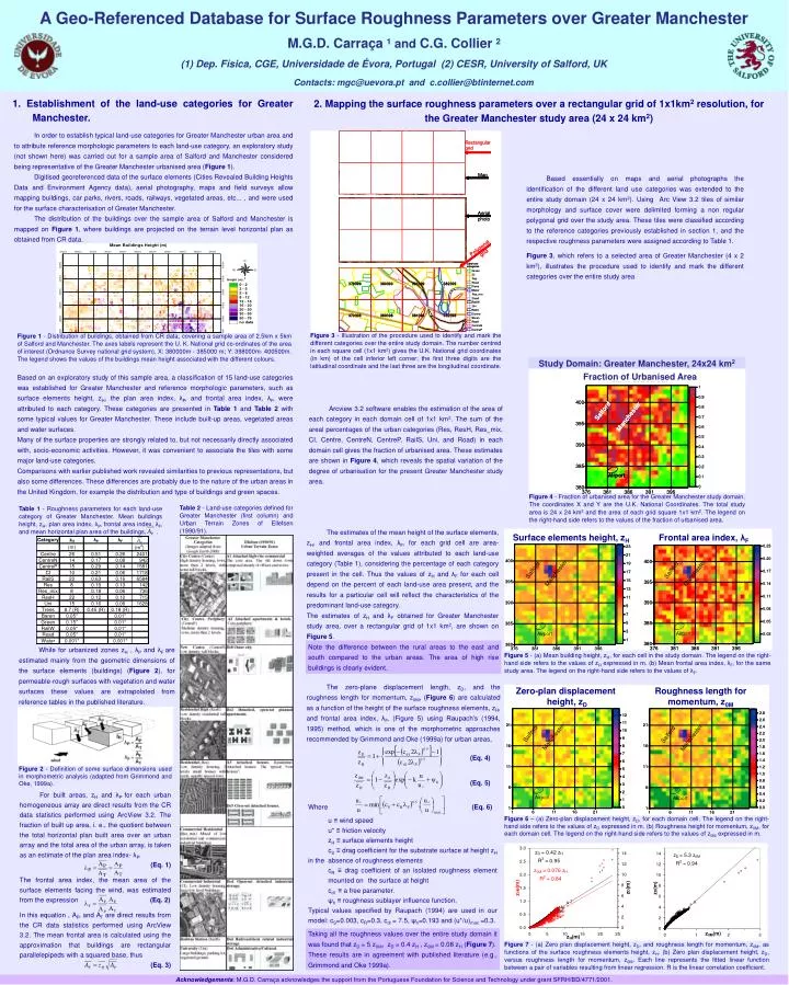
1. A Geo-Referenced Database for Surface Roughness Parameters over Greater Manchester • M.G.D. Carraça1 and C.G. Collier2 • Dep. Física, CGE, Universidade de Évora, Portugal (2) CESR, University of Salford, UK • Contacts: mgc@uevora.pt and c.collier@btinternet.com 1. Establishment of the land-use categories for Greater Manchester. 2. Mapping the surface roughness parameters over a rectangular grid of 1x1km2 resolution, for the Greater Manchester study area (24 x 24 km2) In order to establish typical land-use categories for Greater Manchester urban area and to attribute reference morphologic parameters to each land-use category, an exploratory study (not shown here) was carried out for a sample area of Salford and Manchester considered being representative of the Greater Manchester urbanised area (Figure 1). Digitised georeferenced data of the surface elements (Cities Revealed Building Heights Data and Environment Agency data), aerial photography, maps and field surveys allow mapping buildings, car parks, rivers, roads, railways, vegetated areas, etc... , and were used for the surface characterisation of Greater Manchester. The distribution of the buildings over the sample area of Salford and Manchester is mapped on Figure 1, where buildings are projected on the terrain level horizontal plan as obtained from CR data. Based essentially on maps and aerial photographs the identification of the different land use categories was extended to the entire study domain (24 x 24 km2). Using Arc View 3.2 tiles of similar morphology and surface cover were delimited forming a non regular polygonal grid over the study area. These tiles were classified according to the reference categories previously established in section 1, and the respective roughness parameters were assigned according to Table 1. Figure 3, which refers to a selected area of Greater Manchester (4 x 2 km2), illustrates the procedure used to identify and mark the different categories over the entire study area Fraction of Urbanised Area Figure 3 - Illustration of the procedure used to identify and mark the different categories over the entire study domain. The number centred in each square cell (1x1 km2) gives the U.K. National grid coordinates (in km) of the cell inferior left corner; the first three digits are the latitudinal coordinate and the last three are the longitudinal coordinate. Figure 1 - Distribution of buildings, obtained from CR data, covering a sample area of 2.5km x 5km of Salford and Manchester. The axes labels represent the U. K. National grid co-ordinates of the area of interest (Ordnance Survey national grid system), X: 380000m - 385000 m; Y: 398000m- 400500m. The legend shows the values of the buildings mean height associated with the different colours. Study Domain: Greater Manchester, 24x24 km2 Based on an exploratory study of this sample area, a classification of 15 land-use categories was established for Greater Manchester and reference morphologic parameters, such as surface elements height, zH, the plan area index, λP, and frontal area index, λF, were attributed to each category. These categories are presented in Table 1 and Table 2 with some typical values for Greater Manchester. These include built-up areas, vegetated areas and water surfaces. Many of the surface properties are strongly related to, but not necessarily directly associated with, socio-economic activities. However, it was convenient to associate the tiles with some major land-use categories. Comparisons with earlier published work revealed similarities to previous representations, but also some differences. These differences are probably due to the nature of the urban areas in the United Kingdom, for example the distribution and type of buildings and green spaces. Arcview 3.2 software enables the estimation of the area of each category in each domain cell of 1x1 km2. The sum of the areal percentages of the urban categories (Res, ResH, Res_mix, CI, Centre, CentreN, CentreP, RailS, Uni, and Road) in each domain cell gives the fraction of urbanised area. These estimates are shown in Figure 4, which reveals the spatial variation of the degree of urbanisation for the present Greater Manchester study area. Figure 4 - Fraction of urbanised area for the Greater Manchester study domain. The coordinates X and Y are the U.K. National Coordinates. The total study area is 24 x 24 km2 and the area of each grid square 1x1 km2. The legend on the right-hand side refers to the values of the fraction of urbanised area. Table 2 - Land-use categories defined for Greater Manchester (first column) and Urban Terrain Zones of Ellefsen (1990/91). Table 1 - Roughness parameters for each land-use category of Greater Manchester. Mean buildings height, zH, plan area index, λP, frontal area index, λF, and mean horizontal plan area of the buildings, . The estimates of the mean height of the surface elements, zH, and frontal area index, λF, for each grid cell are area-weighted averages of the values attributed to each land-use category (Table 1), considering the percentage of each category present in the cell. Thus the values of zH and λF for each cell depend on the percent of each land-use area present, and the results for a particular cell will reflect the characteristics of the predominant land-use category. The estimates of zH and λF obtained for Greater Manchester study area, over a rectangular grid of 1x1 km2, are shown on Figure 5. Surface elements height, zH Frontal area index, λF Note the difference between the rural areas to the east and south compared to the urban areas. The area of high rise buildings is clearly evident. While for urbanized zones zH , λP and λF are estimated mainly from the geometric dimensions of the surface elements (buildings) (Figure 2), for permeable-rough surfaces with vegetation and water surfaces these values are extrapolated from reference tables in the published literature. Figure 5 - (a) Mean building height, zH, for each cell in the study domain. The legend on the right-hand side refers to the values of zH expressed in m. (b) Mean frontal area index, λF, for the same study area. The legend on the right-hand side refers to the values of λF. The zero-plane displacement length, zD, and the roughness length for momentum, z0M, (Figure 6) are calculated as a function of the height of the surface roughness elements, zH, and frontal area index, λF, (Figure 5) using Raupach’s (1994, 1995) method, which is one of the morphometric approaches recommended by Grimmond and Oke (1999a) for urban areas, Zero-plan displacement height, zD Roughness length for momentum, z0M (Eq. 4) (Eq. 5) Where (Eq. 6) u ≡ wind speed u* ≡ friction velocity zH ≡ surface elements height cS ≡ drag coefficient for the substrate surface at height zH in the absence of roughness elements cR ≡ drag coefficient of an isolated roughness element mounted on the surface at height cdl ≡ a free parameter. ψh ≡ roughness sublayer influence function, Typical values specified by Raupach (1994) are used in our model: cS=0.003, cR=0.3, cdl = 7.5, ψh=0.193 and (u*/u)max =0.3. Figure 2 - Definition of some surface dimensions used in morphometric analysis (adapted from Grimmond and Oke, 1999a). For built areas, zH and λP for each urban homogeneous array are direct results from the CR data statistics performed using ArcView 3.2. The fraction of built up area, i. e., the quotient between the total horizontal plan built area over an urban array and the total area of the urban array, is taken as an estimate of the plan area index- λP. (Eq. 1) The frontal area index, the mean area of the surface elements facing the wind, was estimated from the expression (Eq. 2) In this equation , AP, and AT are direct results from the CR data statistics performed using ArcView 3.2. The mean frontal area is calculated using the approximation that buildings are rectangular parallelepipeds with a squared base, thus (Eq. 3) Figure 6 – (a) Zero-plan displacement height, zD, for each domain cell. The legend on the right-hand side refers to the values of zD expressed in m. (b) Roughness height for momentum, z0M, for each domain cell. The legend on the right-hand side refers to the values of z0M expressed in m. Taking all the roughness values over the entire study domain it was found that zD = 5 z0M, zD = 0.4 zH , z0M = 0.08 zH (Figure 7). These results are in agreement with published literature (e.g., Grimmond and Oke 1999a). Figure 7 - (a) Zero plan displacement height, zD, and roughness length for momentum, z0M, as functions of the surface roughness elements height, zH. (b) Zero plan displacement height, zD, versus roughness length for momentum, z0M. Each line represents the fitted linear function between a pair of variables resulting from linear regression. R is the linear correlation coefficient. Acknowledgements: M.G.D. Carraça acknowledges the support from the Portuguese Foundation for Science and Technology under grant SFRH/BD/4771/2001.