Download
1 / 29
290 likes | 426 Views
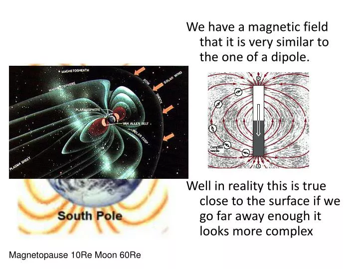
We have a magnetic field that it is very similar to the one of a dipole. Well in reality this is true close to the surface if we go far away enough it looks more complex. Magnetopause 10Re Moon 60Re. Magnetic Field is a vector. It has an intensity (can be measured looking

E N D
We have a magnetic field that it is very similar to the one of a dipole. Well in reality this is true close to the surface if we go far away enough it looks more complex Magnetopause 10Re Moon 60Re
Magnetic Field is a vector It has an intensity (can be measured looking At the oscillation of a compass) And a direction The direction change with the position Magnetic Pole: The place where the compass is pointing down Magnetic Equator: The place where the compass is horizontal
The Earth’s Magnetic Field B = (X, Y, Z) Or B = (F, I, D ) OrB = (D, H, Z) F: intensity I: inclination D: declination H: Horizontal component The seven elements of the (local) magnetic fieldin the geographic coordinate system I. Geomagnetic field – Local Geomagnetic Field Vector
The Earth’s Magnetic Field From this: Magnetic pole is the point where H=0 I= +- 90 Magnetic Equator the point where I=0 F: intensity I: inclination D: declination H: Horizontal component Where 3000nT<H<6000nT erratic zone (compass work badly) Where H<3000nT unusable zone (compass does not work) I. Geomagnetic field – Local Geomagnetic Field Vector
From Press, 1992. 90% of spatial field distribution can be explained by a simple dipolar field
Geomagnetic inclination (IGRF) I. Geomagnetic field – Worldwide Variation of I
Beispiel-Rechnung: Basalt-Probe aus einem gegenwärtigen Ort an 47 S, 20 E. Die remanente Magnetisierung ergibt eine Paleo-Inklination von 30 Grad. Bestimmen wir die Paläolatitude
Position: 47S 20E StereoNet
Position: 47S 20E Declination: N30E
Position: 47S 20E Declination: N30E Inclination: 30 grad Paleolat:16 grad Distance Pole:74 grad
Position: 47S 20E Declination: N30E Inclination: 30 grad Paleolat:16 grad Distance Pole:74 grad
APW Apparent Polar Wander
Since the mechanism of generation of the magnetic field is influenced by the rotation the dipole is mainly oriented along the rotation axis and people use the magnetic pole as past proxy for the rotation axis
PaleoMagnetic Field:Magnetization of Rocks DRM Detrital Remanent Magnetization TRM Thermal Remanent Magnetization
Gesteinsmagnetisierung: Curie Temperatur: etwa 580 Grad C für Magnetit 680 Grad C für Hämatit Blocking Temperatur: Typische Schmelztemperaturen liegen allerdings bei 1100 – 800 Grad C, also wesentlich höher. Das heißt, Gesteine können eine Magnetisierung im Umfeld annehmen, und diese bei Abkühlung unter die Blocking-Temperatur auf geologische Zeiträume hinweg behalten.
Wir unterscheiden: Thermoremanente Magnetisierung: TRM Depositionale Magnetisierung (in Sedimenten): DRM Chemoremanente Magnetisierung: CRM DRM entsteht durch die geordnete Ablagerung magnetischer Minerale in Sedimentgesteinen zur Zeit der Deposition. CRM entsteht durch das langsame Mineralwachstum nach der Ablagerung oder Erstarrung.
A tape recorder “An essay of GeoPoetry” Submarine Lava flow at ridge From www.ridge2000.org/science/tcs/epr06activity.php
A tape recorder “An essay of GeoPoetry” Isochron (or chron)
Chron 13 ~ 34 Ma
Realität: Die Magnetisierung wird nicht in einem infinitesimalen Bereich um den Rücken angenommen. Die Magmenkammern und die Zone vulkanischer Aktivität an einem Rücken, an denen die Magnetisierung stattfindet haben eine Ausdehnungen von mehreren Kilometern (bekannt z.B. durch seismische Messungen). (~5-15 km) (Im Bild: Mit zunehmender Entfernung vom Rücken werden die Krustengesteine Älter. )
Modell mit zeitlicher und räumlicher Zufallsverteilung der Magmenentstehung in Aktivitätszonen unterschiedlicher (10km, 2km, 0km) Weite. Spreizungsrate: 1cm/yr (Atlantik). (i)/(ii)/(iii) 10 Km Aktivitätszone 2 Km “ 0 Km (sog. ideales Blockmodell) Beachte: (i)/(ii)/(iii) ergeben komplexere mag. Anomalien. Jeweils berechnete mag. Anomalien
Berechnung mariner geomagnetischer Anomalien (I): Die theoretische Modellierung magnetischer Anomalien auf dem Ozeanboden ermöglicht es uns, geologische (vergangene) Spreizungsraten aus den heute beobachten Anomalien zu berechnen. Daneben lässt sich aber mit Hilfe der quantitativen Modellierung auch feststellen, ob die Platten ihre Latitude im Laufe der Zeit verändert haben. Dieses Frage ist natürlich der von uns schon behandelten Frage analog, wie man die Paläo-Latitude z.B. von Laven auf den Kontinenten aus Messung remanenter Magnetisierung (z.B. Inklination) bestimmt. Beispiel: Mittelozeanischer Rücken, am Äquator, symmetrische (Ost-West gerichtete) Spreizungsrate; Am Äquator ist die Vertikalkomponente (Z) des Erdmagnetfeldes identisch Null. In diesem Fall ist die permanente Magnetisierung eines idealisierten Blocks am Rücken M=0, My, 0