Download
1 / 1

E N D
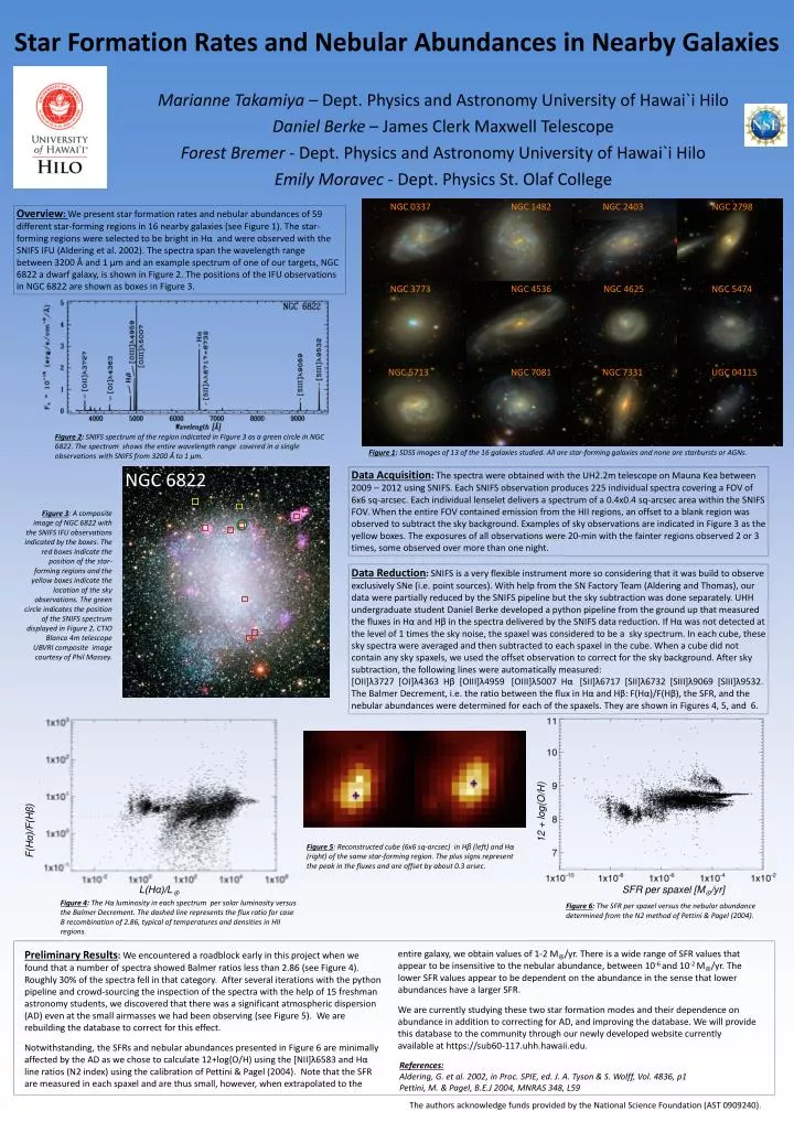
Overview: We present star formation rates and nebular abundances of 59 different star-forming regions in 16 nearby galaxies (see Figure 1). The star-forming regions were selected to be bright in Hαand were observed with theSNIFS IFU (Aldering et al. 2002). The spectra span the wavelength range between 3200 Å and 1 μm and an example spectrum of one of our targets, NGC 6822 a dwarf galaxy, is shown in Figure 2. The positions of the IFU observations in NGC 6822 are shown as boxes in Figure 3. NGC 0337 NGC 1482 NGC 2403 NGC 2798 Star Formation Rates and Nebular Abundances in Nearby Galaxies NGC 6822 NGC 3773 NGC 4536 NGC 4625 NGC 5474 Figure 2: SNIFS spectrum of the region indicated in Figure 3 as a green circle in NGC 6822. The spectrum shows the entire wavelength range covered in a single observations with SNIFS from 3200 Å to 1 μm. Figure 1: SDSS images of 13 of the 16 galaxies studied. All are star-forming galaxies and none are starbursts or AGNs. Data Acquisition: The spectra were obtained with the UH2.2m telescope on Mauna Kea between 2009 – 2012 using SNIFS. Each SNIFS observation produces 225 individual spectra covering a FOV of 6x6 sq-arcsec. Each individual lenselet delivers a spectrum of a 0.4x0.4 sq-arcsec area within the SNIFS FOV. When the entire FOV contained emission from the HII regions, an offset to a blank region was observed to subtract the sky background. Examples of sky observations are indicated in Figure 3 as the yellow boxes. The exposures of all observations were 20-min with the fainter regions observed 2 or 3 times, some observed over more than one night. Figure 3: A composite image of NGC 6822 with the SNIFS IFU observations indicated by the boxes. The red boxes indicate the position of the star-forming regions and the yellow boxes indicate the location of the sky observations. The green circle indicates the position of the SNIFS spectrum displayed in Figure 2. CTIO Blanco 4m telescope UBVRI composite image courtesy of Phil Massey. NGC 5713 NGC 7081 NGC 7331 UGC 04115 Data Reduction: SNIFS is a very flexible instrument more so considering that it was build to observe exclusively SNe (i.e. point sources). With help from the SN Factory Team (Aldering and Thomas), our data were partially reduced by the SNIFS pipeline but the sky subtraction was done separately. UHH undergraduate student Daniel Berke developed a python pipeline from the ground up that measured the fluxes in Hα and Hβ in the spectra delivered by the SNIFS data reduction. If Hα was not detected at the level of 1 times the sky noise, the spaxel was considered to be a sky spectrum. In each cube, these sky spectra were averaged and then subtracted to each spaxel in the cube. When a cube did not contain any sky spaxels, we used the offset observation to correct for the sky background. After sky subtraction, the following lines were automatically measured: [OII]λ3727 [OI]λ4363 Hβ [OIII]λ4959 [OIII]λ5007 Hα [SII]λ6717 [SII]λ6732 [SIII]λ9069 [SIII]λ9532. The Balmer Decrement, i.e. the ratio between the flux in Hα and Hβ: F(Hα)/F(Hβ), the SFR, and the nebular abundances were determined for each of the spaxels. They are shown in Figures 4, 5, and 6. Marianne Takamiya – Dept. Physics and Astronomy University of Hawai`i Hilo Daniel Berke– James Clerk Maxwell Telescope Forest Bremer - Dept. Physics and Astronomy University of Hawai`i Hilo Emily Moravec- Dept. Physics St. Olaf College 12 + log(O/H) F(Hα)/F(Hβ) L(Hα)/L SFR per spaxel [M/yr] Figure 4: The Hα luminosity in each spectrum per solar luminosity versus theBalmer Decrement. The dashed line represents the flux ratio for case B recombination of 2.86, typical of temperatures and densities in HII regions. Figure 6: The SFR per spaxel versus the nebular abundance determined from the N2 method of Pettini & Pagel (2004). Preliminary Results: We encountered a roadblock early in this project when we found that a number of spectra showed Balmer ratios less than 2.86 (see Figure 4). Roughly 30% of the spectra fell in that category. After several iterations with the python pipeline and crowd-sourcing the inspection of the spectra with the help of 15 freshman astronomy students, we discovered that there was a significant atmospheric dispersion (AD) even at the small airmasses we had been observing (see Figure 5). We are rebuilding the database to correct for this effect. Notwithstanding, the SFRs and nebular abundances presented in Figure 6 are minimally affected by the AD as we chose to calculate 12+log(O/H) using the [NII]λ6583 and Hα line ratios (N2 index) using the calibration of Pettini & Pagel (2004). Note that the SFR are measured in each spaxel and are thus small, however, when extrapolated to the entire galaxy, we obtain values of 1-2 M/yr. There is a wide range of SFR values that appear to be insensitive to the nebular abundance, between 10-6 and 10-2 M/yr. The lower SFR values appear to be dependent on the abundance in the sense that lower abundances have a larger SFR. We are currently studying these two starformation modes and their dependence on abundance in addition to correcting for AD, and improving the database. We will provide this database to the community through our newly developed website currently available at https://sub60-117.uhh.hawaii.edu. References: Aldering, G. et al. 2002, in Proc. SPIE, ed. J. A. Tyson & S. Wolff, Vol. 4836, p1 Pettini, M. & Pagel, B.E.J 2004, MNRAS 348, L59 The authors acknowledge funds provided by the National Science Foundation (AST 0909240). Figure 5: Reconstructed cube (6x6 sq-arcsec) in Hβ (left) and Hα (right) of the same star-forming region. The plus signs represent the peak in the fluxes and are offset by about 0.3 arsec.